Videos
(a)
Test whether obese patients has consumed more calories than normal weight siblings or not.
State the test statistic value and make a decision to retain or reject the null hypothesis at 0.05, level of significance.
(a)
Answer to Problem 22CAP
The test statistic value is –1.082.
The decision is to retain the null hypothesis.
The obese patients consumed did not significantly consume more calories than their normal-weight siblings.
Explanation of Solution
The given information is that, sample of 20 obese patientsis considered in which there are two types of sibling are there normal and overweight siblings. The claim is the obese patients consumed significantly more calories than their normal-weight siblings. This represents the alternative hypothesis. The level of significance is 0.05.
The formula of test statistic for one-sample t test is,
In the formula,
Decision rules:
- If the test statistic value is greater than the critical value, then reject the null hypothesis or else retain the null hypothesis.
- If the negative test statistic value is less than negative critical value, then reject the null hypothesis or else retain the null hypothesis.
Let
Null hypothesis:
That is, the obese patients consumed did not significantly consume more calories than their normal-weight siblings.
Alternative hypothesis:
That is, the obese patients consumed significantly consume more calories than their normal-weight siblings.
The degrees of freedom for t distribution is
Critical value:
The given significance level is
The test is one tailed, the degrees of freedom are 9, and the alpha level is 0.05.
From the Appendix B: Table B.2 the t Distribution:
- Locate the value 5 in the degrees of freedom (df) column.
- Locate the 0.05 in the proportion in one tails combined row.
- The intersecting value that corresponds to the 9 with level of significance 0.05 is –1.833.
Thus, the critical value for
Software procedure:
Step by step procedure to obtain test statistic value using SPSS software is given as,
- Choose Variable view.
- Under the name, enter the name as Times.
- Choose Data view, enter the data.
- Choose Analyze>Compare means>Paired Samples T Test.
- In Paired variables, enter the Variable 1 as Normal.
- Enter the Variable 2 as Over.
- Click OK.
Output using SPSS software is given below:
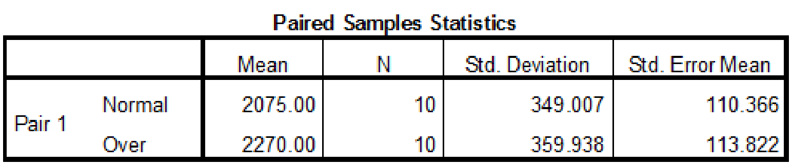
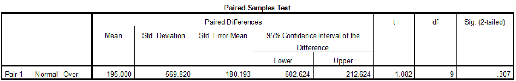
Thus, the test statistic value is –1.082.
Conclusion:
The value of test statistic is –1.082.
The critical value is –1.833.
The test statistic value is greater than the critical value.
The test statistic value does not fall under critical region.
Hence the null hypothesis is retained and obese patients consumed did not significantly consume more calories than their normal-weight siblings.
(b)
Compute effect size using omega-squared.
(b)
Answer to Problem 22CAP
The effect size using omega-squared is 0.02.
Explanation of Solution
Calculations:
From the SPSS output, the test statistic value is –1.082 and
Omega-square:
The proportion of variance is also measured using omega-square. The bias that is caused by eta-square is corrected by omega-squared. The value of omega-square is conservation and give small estimate of proportion of variance. It is denoted by
In the formula, t is the value of test statistic and df is the corresponding degrees of freedom. Subtracting 1 in the numerator reduces the effect size.
The description of effect size using omega-square:
- If value of omega-square is less than 0.01, then effect size is trivial.
- If value of omega-square is in between 0.01 and 0.09, then effect size is small.
- If value of omega-square is in between 0.10 and 0.25, then effect size is medium.
- If value of omega-square is greater than 0.25, then effect size is large.
Substitute,
Thus, the proportion of variance using omega-squared is 0.02. This value is in between 0.01 and 0.09. Hence the Omega-square has a small effect size.
(c)
Explain whether the results support the researcher’s hypothesis or not.
(c)
Answer to Problem 22CAP
No, the results do not support the researcher’s hypothesis.
Explanation of Solution
Justification: The decision of the test is that the obese patients did not consume significantly more calories than their normal-weight siblings. That is, there is no difference in the consumption of calories between obese patients and normal weight siblings.
But the researcher has claimed that ‘the obese patients consumed significantly more calories than their normal-weight siblings’. Hence, the researcher’s hypothesis is not supported.
Want to see more full solutions like this?
Chapter 10 Solutions
Statistics for the Behavioral Sciences


- Please help me with the following question on statisticsFor question (e), the drop down options are: (From this data/The census/From this population of data), one can infer that the mean/average octane rating is (less than/equal to/greater than) __. (use one decimal in your answer).arrow_forwardHelp me on the following question on statisticsarrow_forward3. [15] The joint PDF of RVS X and Y is given by fx.x(x,y) = { x) = { c(x + { c(x+y³), 0, 0≤x≤ 1,0≤ y ≤1 otherwise where c is a constant. (a) Find the value of c. (b) Find P(0 ≤ X ≤,arrow_forwardNeed help pleasearrow_forward7. [10] Suppose that Xi, i = 1,..., 5, are independent normal random variables, where X1, X2 and X3 have the same distribution N(1, 2) and X4 and X5 have the same distribution N(-1, 1). Let (a) Find V(X5 - X3). 1 = √(x1 + x2) — — (Xx3 + x4 + X5). (b) Find the distribution of Y. (c) Find Cov(X2 - X1, Y). -arrow_forward1. [10] Suppose that X ~N(-2, 4). Let Y = 3X-1. (a) Find the distribution of Y. Show your work. (b) Find P(-8< Y < 15) by using the CDF, (2), of the standard normal distribu- tion. (c) Find the 0.05th right-tail percentage point (i.e., the 0.95th quantile) of the distri- bution of Y.arrow_forward6. [10] Let X, Y and Z be random variables. Suppose that E(X) = E(Y) = 1, E(Z) = 2, V(X) = 1, V(Y) = V(Z) = 4, Cov(X,Y) = -1, Cov(X, Z) = 0.5, and Cov(Y, Z) = -2. 2 (a) Find V(XY+2Z). (b) Find Cov(-x+2Y+Z, -Y-2Z).arrow_forward1. [10] Suppose that X ~N(-2, 4). Let Y = 3X-1. (a) Find the distribution of Y. Show your work. (b) Find P(-8< Y < 15) by using the CDF, (2), of the standard normal distribu- tion. (c) Find the 0.05th right-tail percentage point (i.e., the 0.95th quantile) of the distri- bution of Y.arrow_forward== 4. [10] Let X be a RV. Suppose that E[X(X-1)] = 3 and E(X) = 2. (a) Find E[(4-2X)²]. (b) Find V(-3x+1).arrow_forward2. [15] Let X and Y be two discrete RVs whose joint PMF is given by the following table: y Px,y(x, y) -1 1 3 0 0.1 0.04 0.02 I 2 0.08 0.2 0.06 4 0.06 0.14 0.30 (a) Find P(X ≥ 2, Y < 1). (b) Find P(X ≤Y - 1). (c) Find the marginal PMFs of X and Y. (d) Are X and Y independent? Explain (e) Find E(XY) and Cov(X, Y).arrow_forward32. Consider a normally distributed population with mean μ = 80 and standard deviation σ = 14. a. Construct the centerline and the upper and lower control limits for the chart if samples of size 5 are used. b. Repeat the analysis with samples of size 10. 2080 101 c. Discuss the effect of the sample size on the control limits.arrow_forwardConsider the following hypothesis test. The following results are for two independent samples taken from the two populations. Sample 1 Sample 2 n 1 = 80 n 2 = 70 x 1 = 104 x 2 = 106 σ 1 = 8.4 σ 2 = 7.6 What is the value of the test statistic? If required enter negative values as negative numbers (to 2 decimals). What is the p-value (to 4 decimals)? Use z-table. With = .05, what is your hypothesis testing conclusion?arrow_forwardarrow_back_iosSEE MORE QUESTIONSarrow_forward_ios
 Glencoe Algebra 1, Student Edition, 9780079039897...AlgebraISBN:9780079039897Author:CarterPublisher:McGraw Hill
 Big Ideas Math A Bridge To Success Algebra 1: Stu...AlgebraISBN:9781680331141Author:HOUGHTON MIFFLIN HARCOURTPublisher:Houghton Mifflin Harcourt
 Functions and Change: A Modeling Approach to Coll...AlgebraISBN:9781337111348Author:Bruce Crauder, Benny Evans, Alan NoellPublisher:Cengage Learning
 Linear Algebra: A Modern IntroductionAlgebraISBN:9781285463247Author:David PoolePublisher:Cengage Learning