Videos
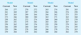
One of the researchers voiced concern about the effect of the new coating on driving distances. Par would like the new cut-resistant ball to offer driving distances comparable to those of the current-model golf ball. To compare the driving distances for the two balls, 40 balls of both the new and current models were subjected to distance tests. The testing was performed with a mechanical hitting machine so that any difference between the mean distances for the two models could be attributed to a difference in the two models. The results of the tests, with distances measured to the nearest yard, follow. These data are available on the website that accompanies the text.
Managerial Report
- 1. Formulate and present the rationale for a hypothesis test that Par could use to compare the driving distances of the current and new golf balls.
- 2. Analyze the data to provide the hypothesis testing conclusion. What is the p-value for your test? What is your recommendation for Par, Inc.?
- 3. Provide
descriptive statistical summaries of the data for each model. - 4. What is the 95% confidence interval for the population mean driving distance of each model, and what is the 95% confidence interval for the difference between the means of the two populations?
- 5. Do you see a need for larger
sample sizes and more testing with the golf balls? Discuss.
1.
State the null and alternative hypothesis.
Answer to Problem 1CP
Null hypothesis:
Alternative hypothesis:
Explanation of Solution
Calculation:
The data represents the results of the tests, with distances measured to the nearest yard for the new model and current model.
Here,
State the hypotheses:
Null hypothesis:
That is, there is no difference between the driving distances of the current and new golf balls.
Alternative hypothesis:
That is, there is a difference between the driving distances of the current and new golf balls.
2.
Find the p-value and provide conclusion.
Answer to Problem 1CP
The p-value is 0.188.
There is sufficient evidence to conclude that, there is no difference between the driving distances of the current and new golf balls.
Explanation of Solution
Calculation:
The test statistic for hypothesis tests about
Software procedure:
Step-by-step software procedure to obtain the confidence interval using MINITAB software is as follows:
- Choose Stat > Basic Statistics > 2 sample t.
- Choose Samples in columns.
- In First column enter Current.
- In Second column enter New.
- Choose Options.
- In Confidence level, enter 95.
- In Alternative, select not equal.
- Click OK in all the dialogue boxes.
Output using MINTAB software is as follows:
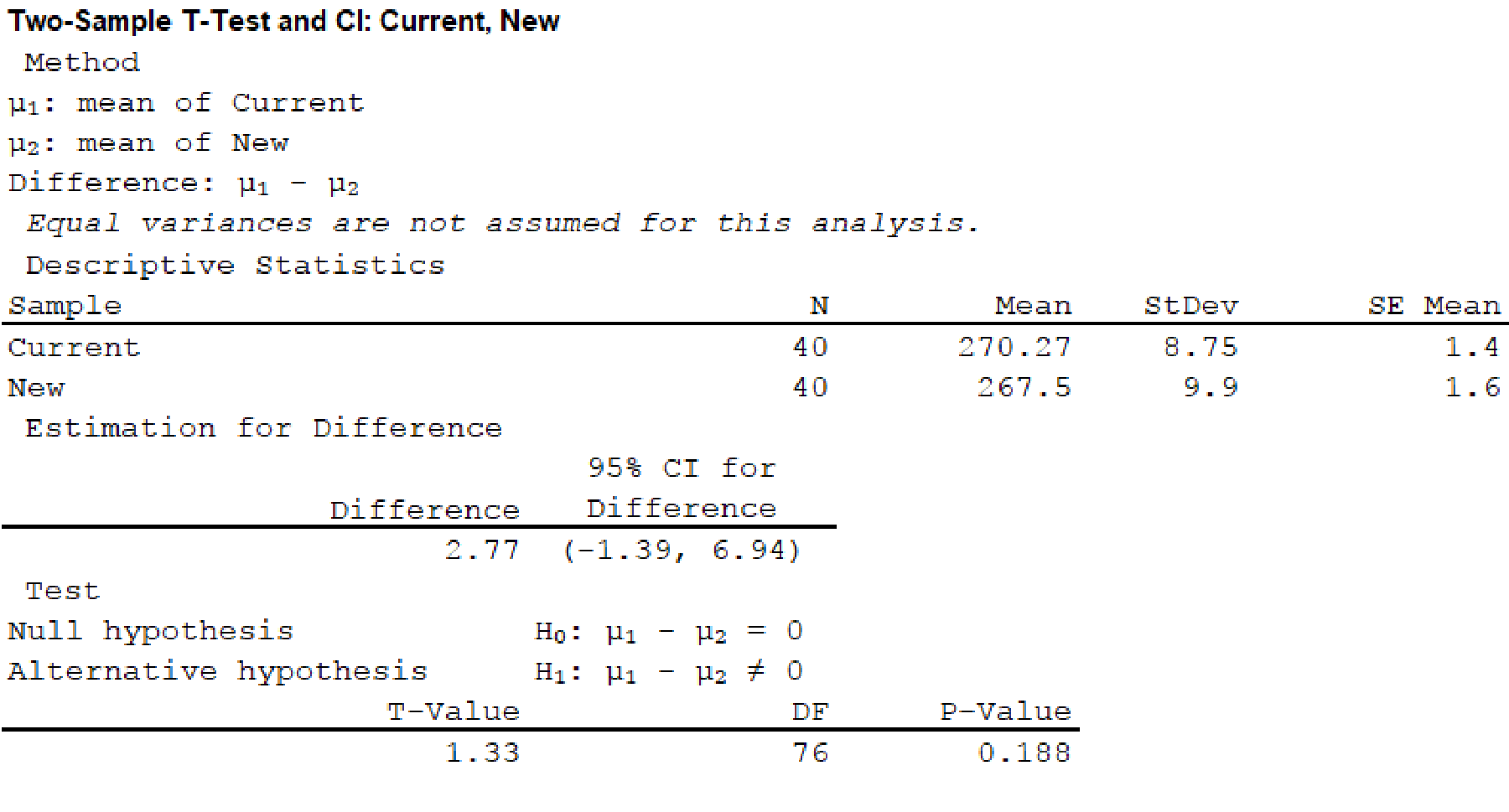
Thus, the test statistic is 1.28 and the p-value is 0.188.
Decision rule based on p-value approach:
If p-value ≤ α, then reject the null hypothesis H0.
If p-value > α, then fail to reject the null hypothesis H0.
Conclusion:
Here, the p-value is 0.188 is greater than the significance level 0.05.
That is,
Thus, the null hypothesis is not rejected.
Therefore, there is sufficient evidence to conclude that, there is no significant difference between the driving distances of the current and new golf balls.
3.
Find the descriptive statistical summaries of the data for each model.
Explanation of Solution
Calculation:
Descriptive statistics for current and new model:
Software procedure:
Step-by-step software procedure to obtain the descriptive statistics using MINITAB software is as follows,
- Choose Stat > Basic Statistics > Display Descriptive Statistics.
- In Variables enter Current and New.
- In Statistics select Mean. SE Mean, StDev, Variance, CoefVar, Q1, Median, Q3, Maximum, IQR.
- Click OK in all the dialogue boxes.
Output using MINITAB software is as follows
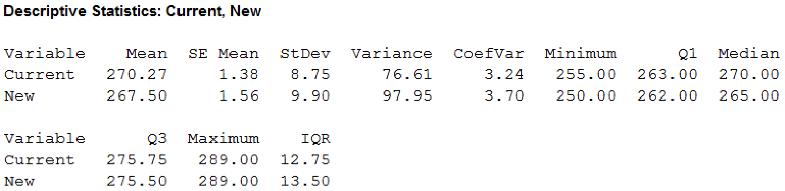
From the output, it can be observed that the mean and median for “current model” is larger than the “new model”. The variance and standard deviation and IQR for “current model” is smaller than “new model”. This indicates that the current model has less variability.
4.
Find the 95% confidence interval for the population mean driving distance of each model.
Find the 95% confidence interval for the difference between the means of the two populations.
Answer to Problem 1CP
The 95% confidence interval for current is
The 95% confidence interval for new is
The 95% confidence interval for the different between the means of the two populations is
Explanation of Solution
Calculation:
Confidence interval for Current:
Software procedure:
Step-by-step software procedure to obtain the confidence interval using MINITAB software is as follows,
- Choose Stat > Basic Statistics > 1 Sample t.
- In Samples in columns enter Current.
- Choose Options.
- In Confidence level, enter 95.
- In Alternative, select not equal.
- Click OK in all the dialogue boxes
Output using MINITAB software is as follows
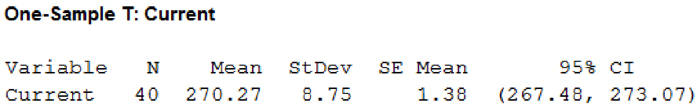
Thus, the 95% confidence interval for current is
Confidence interval for New:
Software procedure:
Step-by-step software procedure to obtain the confidence interval using MINITAB software is as follows,
- Choose Stat > Basic Statistics > 1 Sample t.
- In Samples in columns enter New.
- Choose Options.
- In Confidence level, enter 95.
- In Alternative, select not equal.
- Click OK in all the dialogue boxes
Output using MINITAB software is as follows
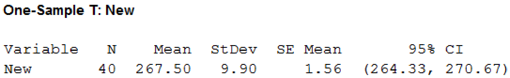
Thus, the 95% confidence interval for new is
Confidence interval for different between the means of the two populations:
Software procedure:
Step-by-step software procedure to obtain the confidence interval using MINITAB software is as follows,
- Choose Stat > Basic Statistics > 2 Sample t.
- Choose Samples in different columns.
- In First enter Current.
- In Second enter New
- Choose Options.
- In Confidence level, enter 95.
- In Alternative, select not equal.
- Click OK in all the dialogue boxes
Output using MINITAB software is as follows
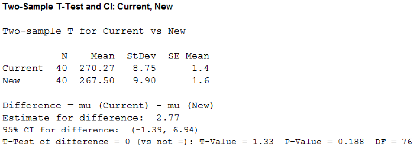
Thus, the 95% confidence interval for the difference between the means of the two populations is
5.
Explain whether there is any need for larger sample sizes and more testing with the golf balls.
Answer to Problem 1CP
No, there is no need for larger sample sizes and there is no need for more testing with the gold balls.
Explanation of Solution
Justification:
From part (2), the null hypothesis not rejected. That is, there is no difference between the driving distances of the current and new golf balls.
Since, the confidence interval for difference between the means of the two populations contains “0” it indicates that there is no difference between the driving distances of the current and new golf balls.
For larger sample size also, the hypotheses test and confidence interval provide the similar results.
Hence, there is need for larger sample sizes and more testing with the golf balls.
Want to see more full solutions like this?
Chapter 10 Solutions
Statistics for Business & Economics, Revised (with XLSTAT Education Edition Printed Access Card)


- Exercise 6-6 (Algo) (LO6-3) The director of admissions at Kinzua University in Nova Scotia estimated the distribution of student admissions for the fall semester on the basis of past experience. Admissions Probability 1,100 0.5 1,400 0.4 1,300 0.1 Click here for the Excel Data File Required: What is the expected number of admissions for the fall semester? Compute the variance and the standard deviation of the number of admissions. Note: Round your standard deviation to 2 decimal places.arrow_forward1. Find the mean of the x-values (x-bar) and the mean of the y-values (y-bar) and write/label each here: 2. Label the second row in the table using proper notation; then, complete the table. In the fifth and sixth columns, show the 'products' of what you're multiplying, as well as the answers. X y x minus x-bar y minus y-bar (x minus x-bar)(y minus y-bar) (x minus x-bar)^2 xy 16 20 34 4-2 5 2 3. Write the sums that represents Sxx and Sxy in the table, at the bottom of their respective columns. 4. Find the slope of the Regression line: bi = (simplify your answer) 5. Find the y-intercept of the Regression line, and then write the equation of the Regression line. Show your work. Then, BOX your final answer. Express your line as "y-hat equals...arrow_forwardApply STATA commands & submit the output for each question only when indicated below i. Generate the log of birthweight and family income of children. Name these new variables Ibwght & Ifaminc. Include the output of this code. ii. Apply the command sum with the detail option to the variable faminc. Note: you should find the 25th percentile value, the 50th percentile and the 75th percentile value of faminc from the output - you will need it to answer the next question Include the output of this code. iii. iv. Use the output from part ii of this question to Generate a variable called "high_faminc" that takes a value 1 if faminc is less than or equal to the 25th percentile, it takes the value 2 if faminc is greater than 25th percentile but less than or equal to the 50th percentile, it takes the value 3 if faminc is greater than 50th percentile but less than or equal to the 75th percentile, it takes the value 4 if faminc is greater than the 75th percentile. Include the outcome of this code…arrow_forward
- solve this on paperarrow_forwardApply STATA commands & submit the output for each question only when indicated below i. Apply the command egen to create a variable called "wyd" which is the rowtotal function on variables bwght & faminc. ii. Apply the list command for the first 10 observations to show that the code in part i worked. Include the outcome of this code iii. Apply the egen command to create a new variable called "bwghtsum" using the sum function on variable bwght by the variable high_faminc (Note: need to apply the bysort' statement) iv. Apply the "by high_faminc" statement to find the V. descriptive statistics of bwght and bwghtsum Include the output of this code. Why is there a difference between the standard deviations of bwght and bwghtsum from part iv of this question?arrow_forwardAccording to a health information website, the distribution of adults’ diastolic blood pressure (in millimeters of mercury, mmHg) can be modeled by a normal distribution with mean 70 mmHg and standard deviation 20 mmHg. b. Above what diastolic pressure would classify someone in the highest 1% of blood pressures? Show all calculations used.arrow_forward
- Write STATA codes which will generate the outcomes in the questions & submit the output for each question only when indicated below i. ii. iii. iv. V. Write a code which will allow STATA to go to your favorite folder to access your files. Load the birthweight1.dta dataset from your favorite folder and save it under a different filename to protect data integrity. Call the new dataset babywt.dta (make sure to use the replace option). Verify that it contains 2,998 observations and 8 variables. Include the output of this code. Are there missing observations for variable(s) for the variables called bwght, faminc, cigs? How would you know? (You may use more than one code to show your answer(s)) Include the output of your code (s). Write the definitions of these variables: bwght, faminc, male, white, motheduc,cigs; which of these variables are categorical? [Hint: use the labels of the variables & the browse command] Who is this dataset about? Who can use this dataset to answer what kind of…arrow_forwardApply STATA commands & submit the output for each question only when indicated below İ. ii. iii. iv. V. Apply the command summarize on variables bwght and faminc. What is the average birthweight of babies and family income of the respondents? Include the output of this code. Apply the tab command on the variable called male. How many of the babies and what share of babies are male? Include the output of this code. Find the summary statistics (i.e. use the sum command) of the variables bwght and faminc if the babies are white. Include the output of this code. Find the summary statistics (i.e. use the sum command) of the variables bwght and faminc if the babies are male but not white. Include the output of this code. Using your answers to previous subparts of this question: What is the difference between the average birthweight of a baby who is male and a baby who is male but not white? What can you say anything about the difference in family income of the babies that are male and male…arrow_forwardA public health researcher is studying the impacts of nudge marketing techniques on shoppers vegetablesarrow_forward
- The director of admissions at Kinzua University in Nova Scotia estimated the distribution of student admissions for the fall semester on the basis of past experience. Admissions Probability 1,100 0.5 1,400 0.4 1,300 0.1 Click here for the Excel Data File Required: What is the expected number of admissions for the fall semester? Compute the variance and the standard deviation of the number of admissions. Note: Round your standard deviation to 2 decimal places.arrow_forwardA pollster randomly selected four of 10 available people. Required: How many different groups of 4 are possible? What is the probability that a person is a member of a group? Note: Round your answer to 3 decimal places.arrow_forwardWind Mountain is an archaeological study area located in southwestern New Mexico. Potsherds are broken pieces of prehistoric Native American clay vessels. One type of painted ceramic vessel is called Mimbres classic black-on-white. At three different sites the number of such sherds was counted in local dwelling excavations. Test given. Site I Site II Site III 63 19 60 43 34 21 23 49 51 48 11 15 16 46 26 20 31 Find .arrow_forward
 Glencoe Algebra 1, Student Edition, 9780079039897...AlgebraISBN:9780079039897Author:CarterPublisher:McGraw Hill
 Big Ideas Math A Bridge To Success Algebra 1: Stu...AlgebraISBN:9781680331141Author:HOUGHTON MIFFLIN HARCOURTPublisher:Houghton Mifflin Harcourt
 Holt Mcdougal Larson Pre-algebra: Student Edition...AlgebraISBN:9780547587776Author:HOLT MCDOUGALPublisher:HOLT MCDOUGAL
 College Algebra (MindTap Course List)AlgebraISBN:9781305652231Author:R. David Gustafson, Jeff HughesPublisher:Cengage Learning