a.
To construct: The
a.
Answer to Problem 10.1.7RE
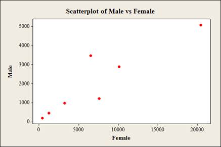
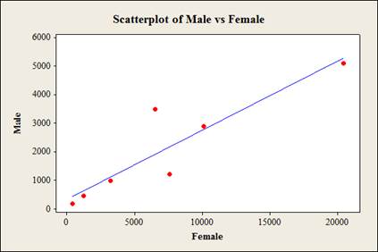
The scatterplot for the data is as follows,
Explanation of Solution
Given info:
The data represents the numbers of male and female physicians.
Calculation:
Software procedure:
Step by step procedure to obtain scatterplot using the MINITAB software:
- Choose Graph > Scatterplot.
- Choose Simple and then click OK.
- Under Y variables, enter a column of Male.
- Under X variables, enter a column of Female.
- Click OK.
b.
To compute: The value of the
b.
Answer to Problem 10.1.7RE
The value of the
Explanation of Solution
Calculation:
Correlation coefficient r:
Software Procedure:
Step-by-step procedure to obtain the ‘correlation coefficient’ using the MINITAB software:
- Select Stat >Basic Statistics > Correlation.
- In Variables, select Male and Female from the box on the left.
- Click OK.
Output using the MINITAB software is given below:
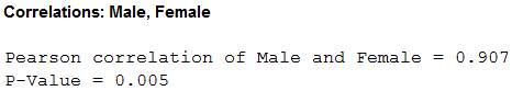
Thus, the value of the correlation is 0.907.
c.
To test: The significance of the correlation coefficient at
c.
Answer to Problem 10.1.7RE
The conclusion is that, there is linear relation between the number of male and female physicians.
Explanation of Solution
Given info:
The level of significance is
Calculation:
The hypotheses are given below:
Null hypothesis:
That is, there is no linear relation between the number of male physicians and number of female physicians.
Alternative hypothesis:
That is, there is a linear relation between the number of male physicians and number of female physicians.
The formula to obtain the degrees of the freedom is
That is,
From the “TABLE –I: Critical Values for the PPMC”, the critical value for 5 degrees of freedom and
Rejection Rule:
If the absolute value of r is greater than the critical value then reject the null hypothesis.
Conclusion:
From part (b), the value of the correlation of Men and Women is 0.907. That is the absolute value of r is 0.907.
Here, the absolute value of r is greater than the critical value.
That is,
By the rejection rule, the null hypothesis is rejected.
Therefore, there is sufficient evidence to support the claim that “there is a linear relation between the number of male and female physicians”.
d.
To find: The regression equation for the given data
d.
Answer to Problem 10.1.7RE
The regression equation for the given data is
Explanation of Solution
Calculation:
Regression:
Software procedure:
Step by step procedure to obtain the regression equation using the MINITAB software:
- Choose Stat > Regression > Regression.
- In Responses, enter the column of Female.
- In Predictors, enter the column of Male.
- Click OK.
Output using the MINITAB software is given below:
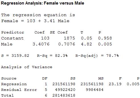
Thus, the regression equation for the given data is
e.
To construct: The regression line on the scatter plot if appropriate.
e.
Answer to Problem 10.1.7RE
The regression line on the scatter plot the scatterplot is as follows,
Explanation of Solution
Calculation:
Step by step procedure to obtain scatterplot using the MINITAB software:
- Choose Graph > Scatterplot.
- Choose With Regression and then click OK.
- Under Y variables, enter a column of Male.
- Under X variables, enter a column of Female.
- Click OK.
f.
To predict: The number of male specialists when there are 2,000 female specialists.
f.
Answer to Problem 10.1.7RE
The predicted value of number of male specialists when there are 2,000 female specialists is 6,923.
Explanation of Solution
From part (d), the regression equation for the given data is
Substitute x as 2,000 in the regression equation
Thus, the predicted value of number of male specialists when there are 2,000 female specialists is 6,923.
Want to see more full solutions like this?
Chapter 10 Solutions
Elementary Statistics: A Step By Step Approach

- Using the accompanying Home Market Value data and associated regression line, Market ValueMarket Valueequals=$28,416plus+$37.066×Square Feet, compute the errors associated with each observation using the formula e Subscript ieiequals=Upper Y Subscript iYiminus−ModifyingAbove Upper Y with caret Subscript iYi and construct a frequency distribution and histogram. Square Feet Market Value1813 911001916 1043001842 934001814 909001836 1020002030 1085001731 877001852 960001793 893001665 884001852 1009001619 967001690 876002370 1139002373 1131001666 875002122 1161001619 946001729 863001667 871001522 833001484 798001589 814001600 871001484 825001483 787001522 877001703 942001485 820001468 881001519 882001518 885001483 765001522 844001668 909001587 810001782 912001483 812001519 1007001522 872001684 966001581 86200arrow_forwarda. Find the value of A.b. Find pX(x) and py(y).c. Find pX|y(x|y) and py|X(y|x)d. Are x and y independent? Why or why not?arrow_forwardThe PDF of an amplitude X of a Gaussian signal x(t) is given by:arrow_forward
- The PDF of a random variable X is given by the equation in the picture.arrow_forwardFor a binary asymmetric channel with Py|X(0|1) = 0.1 and Py|X(1|0) = 0.2; PX(0) = 0.4 isthe probability of a bit of “0” being transmitted. X is the transmitted digit, and Y is the received digit.a. Find the values of Py(0) and Py(1).b. What is the probability that only 0s will be received for a sequence of 10 digits transmitted?c. What is the probability that 8 1s and 2 0s will be received for the same sequence of 10 digits?d. What is the probability that at least 5 0s will be received for the same sequence of 10 digits?arrow_forwardV2 360 Step down + I₁ = I2 10KVA 120V 10KVA 1₂ = 360-120 or 2nd Ratio's V₂ m 120 Ratio= 360 √2 H I2 I, + I2 120arrow_forward
- Q2. [20 points] An amplitude X of a Gaussian signal x(t) has a mean value of 2 and an RMS value of √(10), i.e. square root of 10. Determine the PDF of x(t).arrow_forwardIn a network with 12 links, one of the links has failed. The failed link is randomlylocated. An electrical engineer tests the links one by one until the failed link is found.a. What is the probability that the engineer will find the failed link in the first test?b. What is the probability that the engineer will find the failed link in five tests?Note: You should assume that for Part b, the five tests are done consecutively.arrow_forwardProblem 3. Pricing a multi-stock option the Margrabe formula The purpose of this problem is to price a swap option in a 2-stock model, similarly as what we did in the example in the lectures. We consider a two-dimensional Brownian motion given by W₁ = (W(¹), W(2)) on a probability space (Q, F,P). Two stock prices are modeled by the following equations: dX = dY₁ = X₁ (rdt+ rdt+0₁dW!) (²)), Y₁ (rdt+dW+0zdW!"), with Xo xo and Yo =yo. This corresponds to the multi-stock model studied in class, but with notation (X+, Y₁) instead of (S(1), S(2)). Given the model above, the measure P is already the risk-neutral measure (Both stocks have rate of return r). We write σ = 0₁+0%. We consider a swap option, which gives you the right, at time T, to exchange one share of X for one share of Y. That is, the option has payoff F=(Yr-XT). (a) We first assume that r = 0 (for questions (a)-(f)). Write an explicit expression for the process Xt. Reminder before proceeding to question (b): Girsanov's theorem…arrow_forward
- Problem 1. Multi-stock model We consider a 2-stock model similar to the one studied in class. Namely, we consider = S(1) S(2) = S(¹) exp (σ1B(1) + (M1 - 0/1 ) S(²) exp (02B(2) + (H₂- M2 where (B(¹) ) +20 and (B(2) ) +≥o are two Brownian motions, with t≥0 Cov (B(¹), B(2)) = p min{t, s}. " The purpose of this problem is to prove that there indeed exists a 2-dimensional Brownian motion (W+)+20 (W(1), W(2))+20 such that = S(1) S(2) = = S(¹) exp (011W(¹) + (μ₁ - 01/1) t) 롱) S(²) exp (021W (1) + 022W(2) + (112 - 03/01/12) t). where σ11, 21, 22 are constants to be determined (as functions of σ1, σ2, p). Hint: The constants will follow the formulas developed in the lectures. (a) To show existence of (Ŵ+), first write the expression for both W. (¹) and W (2) functions of (B(1), B(²)). as (b) Using the formulas obtained in (a), show that the process (WA) is actually a 2- dimensional standard Brownian motion (i.e. show that each component is normal, with mean 0, variance t, and that their…arrow_forwardThe scores of 8 students on the midterm exam and final exam were as follows. Student Midterm Final Anderson 98 89 Bailey 88 74 Cruz 87 97 DeSana 85 79 Erickson 85 94 Francis 83 71 Gray 74 98 Harris 70 91 Find the value of the (Spearman's) rank correlation coefficient test statistic that would be used to test the claim of no correlation between midterm score and final exam score. Round your answer to 3 places after the decimal point, if necessary. Test statistic: rs =arrow_forwardBusiness discussarrow_forward
 MATLAB: An Introduction with ApplicationsStatisticsISBN:9781119256830Author:Amos GilatPublisher:John Wiley & Sons Inc
 Probability and Statistics for Engineering and th...StatisticsISBN:9781305251809Author:Jay L. DevorePublisher:Cengage Learning
 Statistics for The Behavioral Sciences (MindTap C...StatisticsISBN:9781305504912Author:Frederick J Gravetter, Larry B. WallnauPublisher:Cengage Learning
 Elementary Statistics: Picturing the World (7th E...StatisticsISBN:9780134683416Author:Ron Larson, Betsy FarberPublisher:PEARSON
 The Basic Practice of StatisticsStatisticsISBN:9781319042578Author:David S. Moore, William I. Notz, Michael A. FlignerPublisher:W. H. Freeman
 Introduction to the Practice of StatisticsStatisticsISBN:9781319013387Author:David S. Moore, George P. McCabe, Bruce A. CraigPublisher:W. H. Freeman