
Concept explainers
Videos
(a)
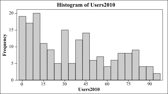
To find: The graphical and numerical summary of the provided data of number of users of internet per 100 people in the year 2010 (Users2010) and to find the numerical summaries of the provided data.
Solution: The obtained histogram indicates that distribution of the data is right skewed. According to the numerical summary, mean of the data is 35.64, minimum value of the data is 0.21, first
(a)
Explanation of Solution
Given: The data of number of users of internet per 100 people (Users2010) is provided in the question.
| Country Name | Users2010 | Users2011 |
| Afghanistan | 3.65 | 4.58 |
| Albania | 45.00 | 49.00 |
| Algeria | 12.50 | 14.00 |
| Andorra | 81.00 | 81.00 |
| Angola | 10.00 | 14.78 |
| Antigua and Barbuda | 80.00 | 82.00 |
| Argentina | 40.00 | 47.70 |
| Aruba | 42.00 | 57.07 |
| Australia | 75.89 | 78.95 |
| Austria | 75.20 | 79.75 |
| Azerbaijan | 46.68 | 50.75 |
| Bahamas, The | 43.00 | 65.00 |
| Bahrain | 55.00 | 77.00 |
| Bangladesh | 3.70 | 5.00 |
| Barbados | 70.20 | 71.77 |
| Belarus | 32.15 | 39.96 |
| Belgium | 73.74 | 76.20 |
| Benin | 3.13 | 3.50 |
| Bermuda | 85.13 | 88.85 |
| Bhutan | 13.60 | 21.00 |
| Bolivia | 22.40 | 30.00 |
| Bosnia and Herzegovina | 52.00 | 60.00 |
| Botswana | 6.00 | 7.00 |
| Brazil | 40.65 | 45.00 |
| Brunei Darussalam | 53.00 | 56.00 |
| Bulgaria | 45.98 | 50.80 |
| Burkina Faso | 2.40 | 3.00 |
| Burundi | 1.00 | 1.11 |
| Cambodia | 1.26 | 3.10 |
| Cameroon | 4.30 | 5.00 |
| Canada | 80.04 | 82.68 |
| Cape Verde | 30.00 | 32.00 |
| Cayman Islands | 66.00 | 69.47 |
| Central African Republic | 2.00 | 2.20 |
| Chad | 1.70 | 1.90 |
| Chile | 45.00 | 53.89 |
| China | 34.39 | 38.40 |
| Colombia | 36.50 | 40.40 |
| Comoros | 5.10 | 5.50 |
| Congo, Dem. Rep. | 0.72 | 1.20 |
| Congo, Rep. | 5.00 | 5.60 |
| Costa Rica | 36.50 | 42.12 |
| Cote d'Ivoire | 2.10 | 2.20 |
| Croatia | 60.12 | 70.53 |
| Cuba | 15.90 | 23.23 |
| Cyprus | 52.99 | 57.68 |
| Czech Republic | 68.64 | 72.89 |
| Denmark | 88.76 | 89.98 |
| Djibouti | 6.50 | 7.00 |
| Dominica | 47.45 | 51.31 |
| Dominican Republic | 31.40 | 35.50 |
| Ecuador | 29.03 | 31.40 |
| Egypt, Arab Rep. | 30.20 | 35.62 |
| El Salvador | 15.90 | 17.69 |
| Eritrea | 5.40 | 6.20 |
| Estonia | 74.15 | 76.53 |
| Ethiopia | 0.75 | 1.10 |
| Faeroe Islands | 75.20 | 80.73 |
| Fiji | 20.00 | 28.00 |
| Finland | 86.91 | 89.33 |
| France | 77.28 | 76.77 |
| French Polynesia | 49.00 | 49.00 |
| Gabon | 7.23 | 8.00 |
| Gambia, The | 9.20 | 10.87 |
| Georgia | 26.29 | 35.28 |
| Germany | 82.53 | 83.44 |
| Ghana | 9.55 | 14.11 |
| Greece | 44.57 | 53.40 |
| Greenland | 63.85 | 64.62 |
| Guatemala | 10.50 | 11.73 |
| Guinea | 1.00 | 1.30 |
| Guinea-Bissau | 2.45 | 2.67 |
| Guyana | 29.90 | 32.00 |
| Honduras | 11.09 | 15.90 |
| Hong Kong SAR, China | 71.85 | 75.03 |
| Hungary | 52.91 | 58.97 |
| Iceland | 95.63 | 96.62 |
| India | 7.50 | 10.07 |
| Indonesia | 10.92 | 18.00 |
| Iran, Islamic Rep. | 16.00 | 21.00 |
| Iraq | 2.47 | 4.95 |
| Ireland | 69.78 | 77.48 |
| Israel | 65.68 | 68.17 |
| Italy | 53.74 | 56.82 |
| Jamaica | 28.07 | 31.99 |
| Japan | 77.65 | 78.71 |
| Jordan | 27.83 | 35.74 |
| Kazakhstan | 31.03 | 44.04 |
| Kenya | 14.00 | 28.00 |
| Kiribati | 9.07 | 10.00 |
| Korea, Rep. | 81.62 | 81.46 |
| Kuwait | 61.40 | 74.20 |
| Kyrgyz Republic | 18.02 | 19.58 |
| Lao PDR | 7.00 | 9.00 |
| Latvia | 68.82 | 72.43 |
| Lebanon | 43.68 | 52.00 |
| Lesotho | 3.86 | 4.22 |
| Liberia | 2.30 | 3.00 |
| Libya | 14.00 | 17.00 |
| Liechtenstein | 80.00 | 85.00 |
| Lithuania | 62.82 | 67.17 |
| Luxembourg | 90.71 | 90.70 |
| Macao SAR, China | 53.80 | 58.00 |
| Macedonia, FYR | 51.90 | 56.70 |
| Madagascar | 1.70 | 1.90 |
| Malawi | 2.26 | 3.33 |
| Malaysia | 56.30 | 61.00 |
| Maldives | 28.30 | 34.00 |
| Mali | 1.90 | 2.00 |
| Malta | 63.08 | 69.03 |
| Mauritania | 4.00 | 4.50 |
| Mauritius | 28.73 | 35.51 |
| Mexico | 31.05 | 36.15 |
| Moldova | 32.40 | 37.85 |
| Mongolia | 12.90 | 20.00 |
| Montenegro | 37.50 | 40.00 |
| Morocco | 49.00 | 51.00 |
| Mozambique | 4.17 | 4.30 |
| Myanmar | 0.25 | 0.98 |
| Namibia | 11.60 | 12.00 |
| Nepal | 7.93 | 9.00 |
| Netherlands | 90.71 | 92.13 |
| New Caledonia | 42.66 | 51.17 |
| New Zealand | 83.01 | 86.18 |
| Nicaragua | 10.00 | 10.60 |
| Niger | 0.83 | 1.30 |
| Nigeria | 24.00 | 28.43 |
| Norway | 93.27 | 93.45 |
| Oman | 62.00 | 68.00 |
| Pakistan | 8.00 | 9.00 |
| Panama | 40.10 | 42.70 |
| Papua New Guinea | 1.28 | 2.00 |
| Paraguay | 19.80 | 23.90 |
| Peru | 34.77 | 36.50 |
| Philippines | 25.00 | 29.00 |
| Poland | 62.47 | 65.02 |
| Portugal | 51.28 | 55.57 |
| Puerto Rico | 45.63 | 48.50 |
| Qatar | 81.60 | 86.20 |
| Romania | 40.02 | 44.12 |
| Russian Federation | 43.31 | 49.31 |
| Rwanda | 8.00 | 7.00 |
| Sao Tome and Principe | 18.75 | 20.16 |
| Saudi Arabia | 41.00 | 47.50 |
| Senegal | 16.00 | 17.50 |
| Serbia | 45.56 | 47.19 |
| Seychelles | 41.00 | 43.61 |
| Singapore | 71.14 | 75.06 |
| Slovak Republic | 76.16 | 74.87 |
| Slovenia | 69.35 | 71.40 |
| Solomon Islands | 5.00 | 6.00 |
| South Africa | 18.05 | 20.95 |
| Spain | 65.81 | 67.92 |
| Sri Lanka | 12.12 | 15.13 |
| St. Lucia | 40.06 | 42.01 |
| St. Vincent and the Grenadines | 38.50 | 43.01 |
| Suriname | 31.59 | 32.00 |
| Swaziland | 12.41 | 20.43 |
| Sweden | 90.01 | 90.88 |
| Switzerland | 82.17 | 82.99 |
| Syrian Arab Republic | 20.66 | 22.44 |
| Tajikistan | 11.55 | 13.03 |
| Tanzania | 11.00 | 12.00 |
| Thailand | 22.40 | 23.70 |
| Timor-Leste | 0.21 | 0.88 |
| Togo | 3.00 | 3.50 |
| Tonga | 16.00 | 25.00 |
| Trinidad and Tobago | 48.50 | 55.20 |
| Tunisia | 36.56 | 38.81 |
| Turkey | 39.82 | 42.10 |
| Turkmenistan | 3.00 | 5.00 |
| Tuvalu | 25.00 | 30.00 |
| Uganda | 12.50 | 13.01 |
| Ukraine | 23.09 | 30.25 |
| United Arab Emirates | 68.00 | 70.00 |
| United Kingdom | 77.75 | 81.71 |
| United States | 74.25 | 78.24 |
| Uruguay | 46.57 | 51.57 |
| Uzbekistan | 19.22 | 28.57 |
| Venezuela, RB | 37.56 | 40.44 |
| Vietnam | 30.97 | 35.45 |
| West Bank and Gaza | 43.44 | 56.82 |
| Yemen, Rep. | 12.35 | 14.91 |
| Zambia | 10.13 | 11.50 |
| Zimbabwe | 11.50 | 15.70 |
Graph: To draw the histogram of the provided data, below mentioned steps are followed in Minitab.
Step 1: Enter the data into Minitab worksheet.
Step 2: Go to Graph, select Histogram and select simple and click OK.
Step 3: Select the data variable column of “Users2010” and click on Scale.
Step 4: Check minor ticks under Y Scale Low and X Scale Low and then click OK.
The obtained histogram is as follows:
Calculation: Use the following steps in Minitab to find the numerical summary for percent users of internet per 100 people.
Step 1. Go to stat option then click on Basis statistics and then choose Display
Step 2. Click on statistics and check minor ticks under Mean, First quartile, Median, Third quartile, Minimum and Maximum.
The numerical summary for percent of users of internet per 100 people in the year 2010 is as follows:
Interpretation: The obtained histogram of the data is plotted and it shows that the data is normal and is right skewed. The mean of the data is 35.64, minimum value of the data is 0.21, first quartile is 10.31, the median is 31.40, third quartile is 55.65 and the maximum value is 95.63.
(b)
To find: The change in number of users per 100 people from 2010 to 2011 and to analyze the changes.
(b)
Answer to Problem 163E
Solution: The minimum value of the data is
Explanation of Solution
Calculation:
Use the following steps in Minitab to find the change in number of users per 100 people from 2010 to 2011.
Step 1. Go to Calc then click on Calculator and enter change in Store result option and enter the formula ‘User2011’-‘User2010’ in the expression option and then click OK.
Step 2. Go to Stat option then click on Basis Statistics and then choose Display Descriptive Statistics.
Step 3. Click on Statistics and check minor ticks under First quartile, Median, Third quartile, Minimum and Maximum.
The numerical summary for change in number of users per 100 people from 2010 to 2011 is as follows:
To draw the histogram of the provided data, below mentioned steps are followed in Minitab.
Step 1: Enter the data into Minitab worksheet.
Step 2: Go to Graph, select Histogram and select simple and click OK.
Step 3: Select the data variable column of “change” and click on Scale.
Step 4: Check minor ticks under Y Scale Low and X Scale Low and then click OK.
The obtained histogram is as follows:
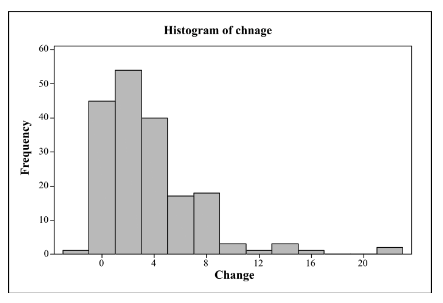
Interpretation: The obtained histogram of the data is plotted and it shows that the data is normal and is left skewed. The minimum value of the data is
(c)
To find: The percent change in number of users per 100 people from 2010 to 2011 and to analyze the changes.
(c)
Answer to Problem 163E
Solution: The minimum value of the data is
Explanation of Solution
Calculation: Use the following steps in Minitab to find the percent change in number of users per 100 people from 2010 to 2011.
Step 1. Go to Calc then click on Calculator and enter % change in Store result option and enter the formula
Step 2. Go to stat option then click on Basis statistics and then choose Display Descriptive Statistics.
Step 3. Click on statistics and check minor ticks under First quartile, Median, Third quartile, Minimum and Maximum.
The numerical summary for change in number of users per 100 people from 2010 to 2011 is as follows:
To draw the histogram of the provided data, below mentioned steps are followed in Minitab.
Step 1: Enter the data into Minitab worksheet.
Step 2: Go to Graph, select Histogram and select simple and click OK.
Step 3: Select the data variable column of “%change” and click on Scale.
Step 4: Check minor ticks under Y Scale Low and X Scale Low and then click OK.
The obtained histogram is as follows:
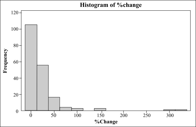
Interpretation: The obtained histogram of the data is plotted and it shows that the data is right skewed. The minimum value of the data is
(d)
The summary to the analysis from part (a) to (c) and to compare between the change and percent change in number of users per 100 people from 2010 to 2011
(d)
Answer to Problem 163E
Solution: Internet utilization has considerably expanded from 2010 to 2011 and the data for internet use in the year 2010 is right skewed.
Explanation of Solution
The data for internet use in the year 2010 is right skewed. The change in internet use from 2010 to 2011 and the percent change are also right skewed. Moreover, there is a gap between the percentage change and it is obtained from the histogram. For every one of the data, numerical summary appears the most ideal approach to depict the distribution. Internet utilization has considerably expanded from 2010 to 2011.
Want to see more full solutions like this?
Chapter 1 Solutions
Introduction to the Practice of Statistics: w/CrunchIt/EESEE Access Card


- PEER REPLY 1: Choose a classmate's Main Post and review their decision making process. 1. Choose a risk level for each of the states of nature (assign a probability value to each). 2. Explain why each risk level is chosen. 3. Which alternative do you believe would be the best based on the maximum EMV? 4. Do you feel determining the expected value with perfect information (EVWPI) is worthwhile in this situation? Why or why not?arrow_forwardQuestions An insurance company's cumulative incurred claims for the last 5 accident years are given in the following table: Development Year Accident Year 0 2018 1 2 3 4 245 267 274 289 292 2019 255 276 288 294 2020 265 283 292 2021 263 278 2022 271 It can be assumed that claims are fully run off after 4 years. The premiums received for each year are: Accident Year Premium 2018 306 2019 312 2020 318 2021 326 2022 330 You do not need to make any allowance for inflation. 1. (a) Calculate the reserve at the end of 2022 using the basic chain ladder method. (b) Calculate the reserve at the end of 2022 using the Bornhuetter-Ferguson method. 2. Comment on the differences in the reserves produced by the methods in Part 1.arrow_forwardYou are provided with data that includes all 50 states of the United States. Your task is to draw a sample of: o 20 States using Random Sampling (2 points: 1 for random number generation; 1 for random sample) o 10 States using Systematic Sampling (4 points: 1 for random numbers generation; 1 for random sample different from the previous answer; 1 for correct K value calculation table; 1 for correct sample drawn by using systematic sampling) (For systematic sampling, do not use the original data directly. Instead, first randomize the data, and then use the randomized dataset to draw your sample. Furthermore, do not use the random list previously generated, instead, generate a new random sample for this part. For more details, please see the snapshot provided at the end.) Upload a Microsoft Excel file with two separate sheets. One sheet provides random sampling while the other provides systematic sampling. Excel snapshots that can help you in organizing columns are provided on the next…arrow_forward
- The population mean and standard deviation are given below. Find the required probability and determine whether the given sample mean would be considered unusual. For a sample of n = 65, find the probability of a sample mean being greater than 225 if μ = 224 and σ = 3.5. For a sample of n = 65, the probability of a sample mean being greater than 225 if μ=224 and σ = 3.5 is 0.0102 (Round to four decimal places as needed.)arrow_forward***Please do not just simply copy and paste the other solution for this problem posted on bartleby as that solution does not have all of the parts completed for this problem. Please answer this I will leave a like on the problem. The data needed to answer this question is given in the following link (file is on view only so if you would like to make a copy to make it easier for yourself feel free to do so) https://docs.google.com/spreadsheets/d/1aV5rsxdNjHnkeTkm5VqHzBXZgW-Ptbs3vqwk0SYiQPo/edit?usp=sharingarrow_forwardThe data needed to answer this question is given in the following link (file is on view only so if you would like to make a copy to make it easier for yourself feel free to do so) https://docs.google.com/spreadsheets/d/1aV5rsxdNjHnkeTkm5VqHzBXZgW-Ptbs3vqwk0SYiQPo/edit?usp=sharingarrow_forward
- The following relates to Problems 4 and 5. Christchurch, New Zealand experienced a major earthquake on February 22, 2011. It destroyed 100,000 homes. Data were collected on a sample of 300 damaged homes. These data are saved in the file called CIEG315 Homework 4 data.xlsx, which is available on Canvas under Files. A subset of the data is shown in the accompanying table. Two of the variables are qualitative in nature: Wall construction and roof construction. Two of the variables are quantitative: (1) Peak ground acceleration (PGA), a measure of the intensity of ground shaking that the home experienced in the earthquake (in units of acceleration of gravity, g); (2) Damage, which indicates the amount of damage experienced in the earthquake in New Zealand dollars; and (3) Building value, the pre-earthquake value of the home in New Zealand dollars. PGA (g) Damage (NZ$) Building Value (NZ$) Wall Construction Roof Construction Property ID 1 0.645 2 0.101 141,416 2,826 253,000 B 305,000 B T 3…arrow_forwardRose Par posted Apr 5, 2025 9:01 PM Subscribe To: Store Owner From: Rose Par, Manager Subject: Decision About Selling Custom Flower Bouquets Date: April 5, 2025 Our shop, which prides itself on selling handmade gifts and cultural items, has recently received inquiries from customers about the availability of fresh flower bouquets for special occasions. This has prompted me to consider whether we should introduce custom flower bouquets in our shop. We need to decide whether to start offering this new product. There are three options: provide a complete selection of custom bouquets for events like birthdays and anniversaries, start small with just a few ready-made flower arrangements, or do not add flowers. There are also three possible outcomes. First, we might see high demand, and the bouquets could sell quickly. Second, we might have medium demand, with a few sold each week. Third, there might be low demand, and the flowers may not sell well, possibly going to waste. These outcomes…arrow_forwardConsider the state space model X₁ = §Xt−1 + Wt, Yt = AX+Vt, where Xt Є R4 and Y E R². Suppose we know the covariance matrices for Wt and Vt. How many unknown parameters are there in the model?arrow_forward
- Business Discussarrow_forwardYou want to obtain a sample to estimate the proportion of a population that possess a particular genetic marker. Based on previous evidence, you believe approximately p∗=11% of the population have the genetic marker. You would like to be 90% confident that your estimate is within 0.5% of the true population proportion. How large of a sample size is required?n = (Wrong: 10,603) Do not round mid-calculation. However, you may use a critical value accurate to three decimal places.arrow_forward2. [20] Let {X1,..., Xn} be a random sample from Ber(p), where p = (0, 1). Consider two estimators of the parameter p: 1 p=X_and_p= n+2 (x+1). For each of p and p, find the bias and MSE.arrow_forward
 Glencoe Algebra 1, Student Edition, 9780079039897...AlgebraISBN:9780079039897Author:CarterPublisher:McGraw Hill
 Holt Mcdougal Larson Pre-algebra: Student Edition...AlgebraISBN:9780547587776Author:HOLT MCDOUGALPublisher:HOLT MCDOUGAL
 College Algebra (MindTap Course List)AlgebraISBN:9781305652231Author:R. David Gustafson, Jeff HughesPublisher:Cengage Learning
 Big Ideas Math A Bridge To Success Algebra 1: Stu...AlgebraISBN:9781680331141Author:HOUGHTON MIFFLIN HARCOURTPublisher:Houghton Mifflin Harcourt
 Functions and Change: A Modeling Approach to Coll...AlgebraISBN:9781337111348Author:Bruce Crauder, Benny Evans, Alan NoellPublisher:Cengage Learning
 Algebra: Structure And Method, Book 1AlgebraISBN:9780395977224Author:Richard G. Brown, Mary P. Dolciani, Robert H. Sorgenfrey, William L. ColePublisher:McDougal Littell