Chapter 1, Problem 13CE

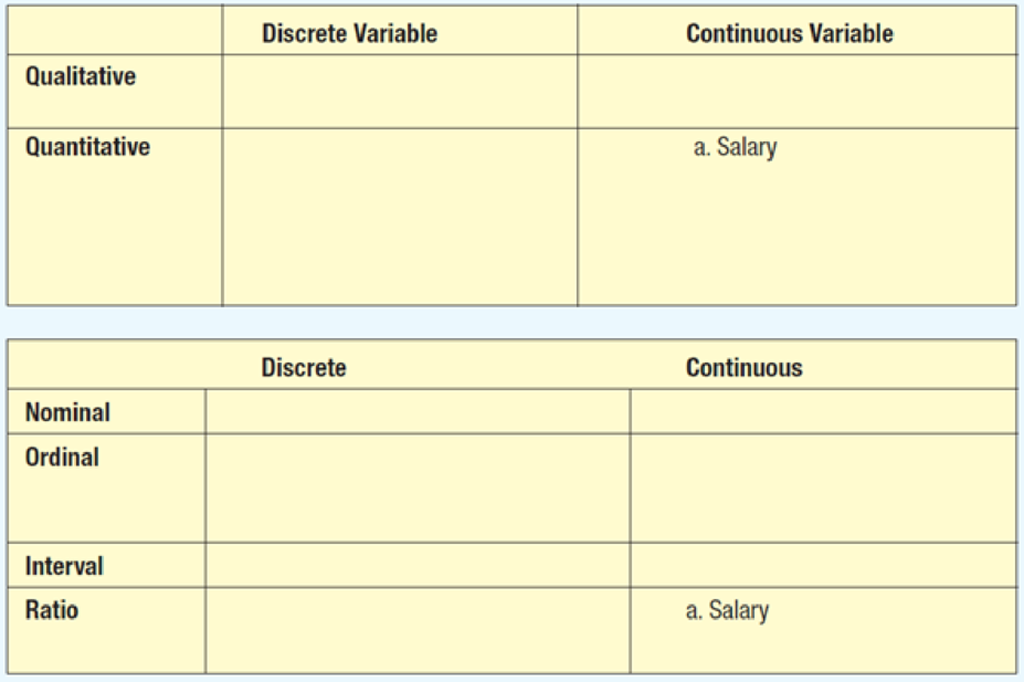
Place these variables in the following classification tables. For each table, summarize your observations and evaluate if the results are generally true. For example, salary is reported as a continuous quantitative variable. It is also a continuous ratio-scaled variable.

1. a. Salary
2. b. Gender
3. c. Sales volume of MP3 players
4. d. Soft drink preference
5. e. Temperature
6. f. SAT scores
7. g. Student rank in class
8. h. Rating of a finance professor
9. i. Number of home computers

To determine

Classify each variable as discrete or continuous, qualitative or quantitative, nominal or ordinal or interval or ratio, and put them into the given tables.

Answer to Problem 13CE

The classifications of the variables in the tables are as follows:

	Discrete	Continuous
Qualitative	b. Gender d. Soft drink preference g. Student rank in class h. Rating of a finance professor
Quantitative	c. Sales volume of MP3 players f. SAT scores i. Number of home computers	a. Salary e. Temperature

	Discrete	Continuous
Nominal	b. Gender
Ordinal	d. Soft drink preference g. Student rank in class h. Rating of a finance professor
Interval	f. SAT scores	e. Temperature
Ratio	c. Sales volume of MP3 players i. Number of home computers	a. Salary

Explanation of Solution

Classification type Qualitative or quantitative:

Qualitative variable:

A qualitative variable, also called an attribute, is defined as the characteristic of an entity, which naturally takes non-numeric values. The values of a qualitative variable are usually categories. Even if such a variable happens to take numeric values, it would be simply as a label or a tag, on which, no arithmetic operations can be logically performed, other that counting the number of observations in each category and the corresponding percentages.

Quantitative variable:

A quantitative variable is defined as the characteristic of an entity, which naturally takes numeric values. It is logical to perform at least one arithmetic operation, such as addition, subtraction, multiplication, division, etc. on a quantitative variable.

Classification type: Discrete or continuous:

Discrete variable:

A discrete variable is defined as the quantitative variable corresponding to a characteristic of an entity that can take only some distinct numeric values in a given range. Within two consecutive distinct values, there is usually a gap, such that no observation can take a value in that gap. A discrete variable is usually “counted”.

Continuous variable:

A continuous variable is defined as the quantitative variable corresponding to a characteristic of an entity that can take any numeric values within a given range. It is not necessary to have a fixed gap within any two consecutive continuous variable values. A continuous variable is usually “measured”.

Classification type: Levels of measurement:

Nominal level of measurement:

A variable is said to be recorded at the nominal level of measurement, if its values comprise only of names and labels, which do not have any natural order and can only be counted.

Ordinal level of measurement:

A variable is said to be recorded at the ordinal level of measurement, if its values comprise of names and labels, which occur in a natural order and can only be counted.

Interval level of measurement:

A variable is said to be recorded at the interval level of measurement, if its values comprise of numbers or levels, in which, the distance between any two values is meaningfully defined, and the scale of measurement has a known unit.

Ratio level of measurement:

A variable is said to be recorded at the ratio level of measurement, if its values comprise of numbers, among which, the value zero is absolutely defined, and the scale of measurement has a known unit.

a. Salary:

The salary of an individual can take numerical values, on which, it is logical to perform arithmetic operation. Thus, salary is a quantitative variable.

The salary can take any numerical value within a given range. It is not necessary for the salary to be distinct numbers. Thus, salary is a continuous variable.

The salary takes numerical values, with units such as dollars. Moreover, the value 0 of salary is absolute, which implies that an individual receives no salary, and which is logical. Thus, salary is at the ratio level of measurement.

b. Gender:

The gender of an individual cannot take numerical values. On these values, it is not logical to perform arithmetic operation. Thus, gender is a qualitative variable.

The gender can be any one of several distinct categories. It cannot take any value within a given range. Thus, gender is a discrete variable.

The gender takes non-numerical values, with no units. The values of the variable gender are simply labels or tags, which are not numerical. Thus, gender is at the nominal level of measurement.

c. Sales volume of MP3 players:

The sales volume of MP3 players can take numerical values, on which, it is logical to perform arithmetic operation. Thus, sales volume of MP3 players is a quantitative variable.

The sales volume of MP3 players can take only some distinct numerical value within a given range. It can be counted, and cannot take any value within a given range. Thus, sales volume of MP3 players is a continuous variable.

The sales volume of MP3 players takes numerical values. Moreover, the value 0 of sales volume of MP3 players is absolute, which implies that there was no sale of MP3 players at a certain store, and which is logical. Thus, sales volume of MP3 players is at the ratio level of measurement.

d. Soft drink preference:

The soft drink preference of an individual cannot take numerical values. On these values, it is not logical to perform arithmetic operation. Thus, soft drink preference is a qualitative variable.

The soft drink preference can be any one of several distinct categories. It cannot take any value within a given range. Thus, soft drink preference is a discrete variable.

The soft drink preference takes non-numerical values, with no units. The values of the variable are simply labels or tags, which can have a natural order, based on the level of preference. Thus, soft drink preference is at the ordinal level of measurement.

e. Temperature:

The temperature can take numerical values, on which, it is logical to perform arithmetic operation. Thus, temperature is a quantitative variable.

The temperature can take any numerical value within a given range. It is not necessary for the temperature to be distinct numbers. Thus, temperature is a continuous variable.

The temperature takes numerical values, with units such as Celsius, Fahrenheit, Kelvin, etc. However, the value 0 of temperature is not absolute; a temperature of 0 on one scale corresponds to a non-zero temperature on another one. Thus, temperature is at the interval level of measurement.

f. SAT scores:

The SAT scores of an individual can take numerical values, on which, it is logical to perform arithmetic operation. Thus, SAT scores is a quantitative variable.

The SAT scores of students can take only some distinct values, and not just any value within a given range. It cannot take any value within a given range. Thus, SAT scores are a discrete variable.

The SAT scores take numerical. However, Moreover the value 0 of SAT scores is not absolute, and not logical. Moreover, the ratio of two SAT scores is illogical. Thus, SAT scores are at the interval level of measurement.

g. Student rank in class:

The student rank in class of an individual cannot take numerical values. On these values, it is not logical to perform arithmetic operation. Thus, student rank in class is a qualitative variable.

The student rank in class can be any one of several distinct categories. It cannot take any value within a given range. Thus, student rank in class is a discrete variable.

The student rank in class takes non-numerical values, with no units. The values of the variable are simply labels or tags, which can have a natural order, based on the class performance of the student. Thus, student rank in class is at the ordinal level of measurement.

h. Rating of a finance professor:

The rating of a finance professor cannot take numerical values. On these values, it is not logical to perform arithmetic operation. Thus, rating of a finance professor is a qualitative variable.

The rating of a finance professor can be any one of several distinct categories. It cannot take any value within a given range. Thus, rating of a finance professor is a discrete variable.

The rating of a finance professor takes non-numerical values, with no units, unless otherwise mentioned. The values of the variable are simply labels or tags, which can have a natural order, based on the level of liking for the professor. Thus, rating of a finance professor is at the ordinal level of measurement.

i. Number of home computers:

The number of home computers in a home can take numerical values, on which, it is logical to perform arithmetic operation. Thus, number of home computers is a quantitative variable.

The number of home computers can take only some distinct numerical value within a given range. It can be counted, and cannot take any value within a given range. Thus, number of home computers is a continuous variable.

The number of home computers takes numerical values. Moreover, the value 0 of number of home computers is absolute, which implies that a home has no home computers, and which is logical. Thus, number of home computers is at the ratio level of measurement.