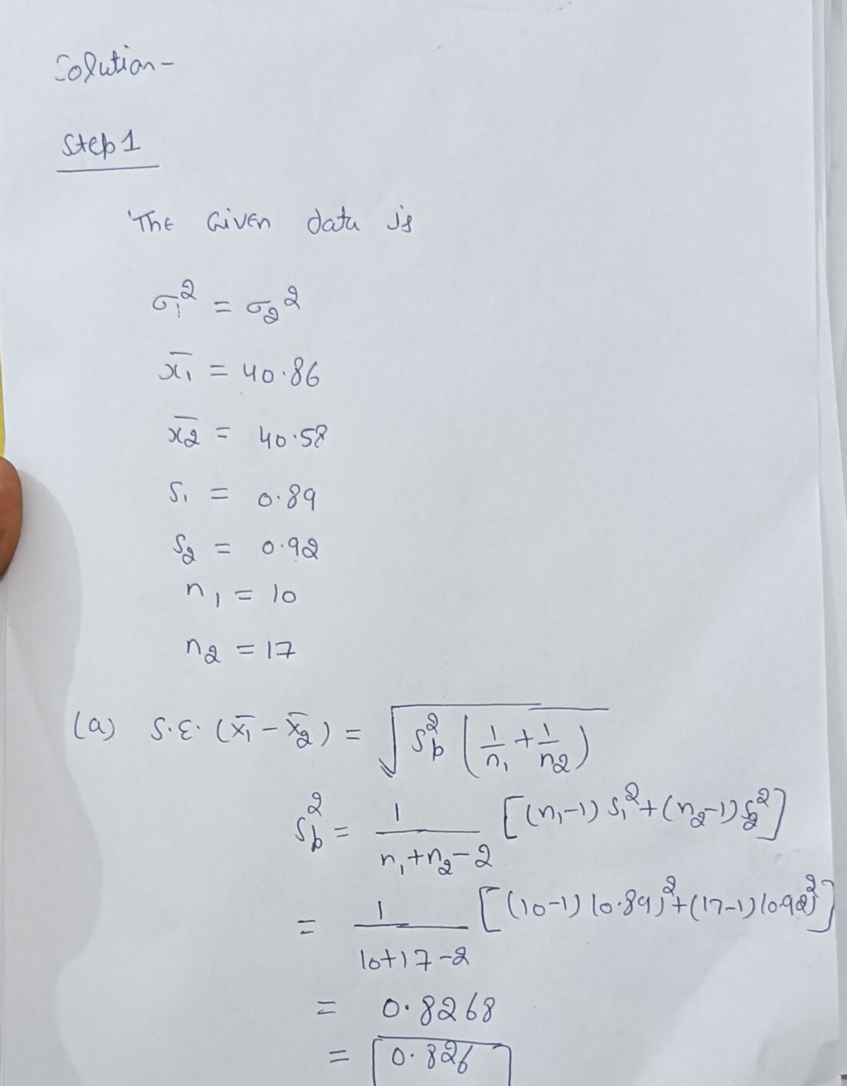
Tests the claim that #1 # p2. Assume the samples are normally distributed, random and independent. of = o} %3D s1 = 0.89 ; s2 = 0.92 = 40.86; zz = 40.58 n = 10; n2 = 17 a. Calculate the Standard Error s - = (use 3 decimals) b. Calculate the t-test statistic using the standard error from part a. t = (use 2 decimal places) c. What are the degrees of freedom? df = d. At a = 0.05 , Use the distribution table to find the critical values for the rejection region te = ± (use 4 decimal places) e. What is your conclusion? O Accept the alternative hypothesis and reject the claim O Accept the null hypothesis and support the claim O Fail to reject the null hypothesis and do not support the claim O Reject the null hypothesis and support the claim O Reject the alternative hypothesis and support the claim
Tests the claim that #1 # p2. Assume the samples are normally distributed, random and independent. of = o} %3D s1 = 0.89 ; s2 = 0.92 = 40.86; zz = 40.58 n = 10; n2 = 17 a. Calculate the Standard Error s - = (use 3 decimals) b. Calculate the t-test statistic using the standard error from part a. t = (use 2 decimal places) c. What are the degrees of freedom? df = d. At a = 0.05 , Use the distribution table to find the critical values for the rejection region te = ± (use 4 decimal places) e. What is your conclusion? O Accept the alternative hypothesis and reject the claim O Accept the null hypothesis and support the claim O Fail to reject the null hypothesis and do not support the claim O Reject the null hypothesis and support the claim O Reject the alternative hypothesis and support the claim

MATLAB: An Introduction with Applications
6th Edition
ISBN:9781119256830
Author:Amos Gilat
Publisher:Amos Gilat
Chapter1: Starting With Matlab
Section: Chapter Questions
Problem 1P

Related questions
Question

Transcribed Image Text:Tests the claim that #1 # p2. Assume the samples are normally distributed, random and independent.
of = o}
%3D
s1 = 0.89 ; s2 = 0.92
I1 = 40.86 ; z2 = 40.58
n1 = 10; n2 = 17
a. Calculate the Standard Error si-i, =
(use 3 decimals)
b. Calculate the t-test statistic using the standard error from part a. t =
(use 2 decimal places)
c. What are the degrees of freedom? df =
d. At a = 0.05 , Use the distribution table to find the critical values for the rejection region
te = ±
(use 4 decimal places)
e. What is your conclusion?
O Accept the alternative hypothesis and reject the claim
O Accept the null hypothesis and support the claim
O Fail to reject the null hypothesis and do not support the claim
O Reject the null hypothesis and support the claim
O Reject the alternative hypothesis and support the claim
Expert Solution
Step 1
Solution

Step by step
Solved in 2 steps with 2 images

Recommended textbooks for you
MATLAB: An Introduction with Applications
Statistics
ISBN:
9781119256830
Author:
Amos Gilat
Publisher:
John Wiley & Sons Inc

Probability and Statistics for Engineering and th…
Statistics
ISBN:
9781305251809
Author:
Jay L. Devore
Publisher:
Cengage Learning

Statistics for The Behavioral Sciences (MindTap C…
Statistics
ISBN:
9781305504912
Author:
Frederick J Gravetter, Larry B. Wallnau
Publisher:
Cengage Learning
MATLAB: An Introduction with Applications
Statistics
ISBN:
9781119256830
Author:
Amos Gilat
Publisher:
John Wiley & Sons Inc
Probability and Statistics for Engineering and th…
Statistics
ISBN:
9781305251809
Author:
Jay L. Devore
Publisher:
Cengage Learning
Statistics for The Behavioral Sciences (MindTap C…
Statistics
ISBN:
9781305504912
Author:
Frederick J Gravetter, Larry B. Wallnau
Publisher:
Cengage Learning

Elementary Statistics: Picturing the World (7th E…
Statistics
ISBN:
9780134683416
Author:
Ron Larson, Betsy Farber
Publisher:
PEARSON

The Basic Practice of Statistics
Statistics
ISBN:
9781319042578
Author:
David S. Moore, William I. Notz, Michael A. Fligner
Publisher:
W. H. Freeman

Introduction to the Practice of Statistics
Statistics
ISBN:
9781319013387
Author:
David S. Moore, George P. McCabe, Bruce A. Craig
Publisher:
W. H. Freeman