Summary of Fit RSquare RSquare Adj Root Mean Square Error Mean of Response Observations (or Sum Wgts) 0.939928 0.927413 0.18139 8.382667 30 Analysis of Variance Sum of Mean Source DF Squares Square 2.47113 F Ratio Model 5 12.355673 75.1044 Error 24 0.789664 0.03290 Prob > F C. Total 29 13.145337 <.0001* Estimate Prob>|t| t Ratio 4.10 -4.83 Lower 95% Upper 95% 10.774546 Term Std Error Intercept Price(X1) IndPrice(X2) AdvExp(X3) 7.169166 1.746879 0.0004050* 3.5637864 <0.0001* <0.0001* -2.265398 0.468984 -3.23333 -1.297463 1.4060571 0.219462 6.41 0.9531107 1.8590036 ו0.77793 0.4905504 0.5953108 0.088483 6.73 <0.0001* 0.412692 0.0010047* <0.0001* DB 0.316214 0.084470 3.74 0.1418769 DC 0.5245297 0.086988 6.03 0.3449961 0.7040632 Upper 95% Mean Demand 8.767117947 Upper 95% Indiv Demand Predicted Lower 95% Lower 95% Demand Mean Demand Indiv Demand 31 8.641889387 8.516660827 8.247127546 9.836651228 = 89 + 81 1 + 82 2 + 83 a3 + 8gDs + @5Dc + e Click here for the Excel Data File a) In this model the parameter 64 represents the effect on mean demand of advertising campaign B compared to advertising campaign A, and the parameter 65 represents the effect on mean demand of advertising campaign C compared to advertising campaign A. Use the regression output to find and report a point estimate of each of the above effects and to test the significance c each of the above effects. Also, find and report a 95 percent confidence interval for each of the above effects. Interpret your results Round your answers to 4 decimal places.) The point estimate of the effect on the mean of campaign B compared to campaign A is b4 = The 95% confidence interval = [ 1. The point estimate of the effect on the mean of campaign C compared to campaign A is b5 = 1. The 95% confidence interval = [ Campaign is probably most effective even though intervals overlap.


Ch 13. 3:
Enterprise Industries produces Fresh, a brand of liquid laundry detergent. In order to manage its inventory more effectively and make revenue projections, the company would like to better predict demand for Fresh. To develop a prediction model, the company has gathered data concerning demand for Fresh over the last 30 sales periods (each sales period is defined to be a four-week period). The demand data are presented in table below concerning y (demand for Fresh liquid laundry detergent), x1 (the price of Fresh), x2 (the average industry price of competitors' similar detergents), and x3 (Enterprise Industries’ advertising expenditure for Fresh). To ultimately increase the demand for Fresh, Enterprise Industries’ marketing department is comparing the effectiveness of three different advertising campaigns. These campaigns are denoted as campaigns A, B, and C. Campaign A consists entirely of television commercials, campaign B consists of a balanced mixture of television and radio commercials, and campaign C consists of a balanced mixture of television, radio, newspaper, and magazine ads. To conduct the study, Enterprise Industries has randomly selected one advertising campaign to be used in each of the 30 sales periods in table below. Although logic would indicate that each of campaigns A, B, and C should be used in 10 of the 30 sales periods, Enterprise Industries has made previous commitments to the advertising media involved in the study. As a result, campaigns A, B, and C were randomly assigned to, respectively, 9, 11, and 10 sales periods. Furthermore, advertising was done in only the first three weeks of each sales period, so that the carryover effect of the campaign used in a sales period to the next sales period would be minimized. Table lists the campaigns used in the sales periods.
To compare the effectiveness of advertising campaigns A, B, and C, we define two dummy variables. Specifically, we define the dummy variable DB to equal 1 if campaign B is used in a sales period and 0 otherwise. Furthermore, we define the dummy variable DC to equal 1 if campaign C is used in a sales period and 0 otherwise. Table presents the JMP output of a
| Historical Data Concerning Demand for Fresh Detergent | ||||
| Sales Period |
Price for Fresh, x1 |
Average Industry Price, x2 |
Advertising Expenditure for Fresh, x3 |
Demand for Fresh, y |
| 1 | 3.96 | 3.83 | 5.52 | 7.31 |
| 2 | 3.79 | 4.05 | 6.78 | 8.52 |
| 3 | 3.75 | 4.35 | 7.22 | 9.23 |
| 4 | 3.70 | 3.78 | 5.56 | 7.50 |
| 5 | 3.62 | 3.88 | 7.03 | 9.31 |
| 6 | 3.62 | 3.88 | 6.59 | 8.24 |
| 7 | 3.67 | 3.79 | 6.79 | 8.73 |
| 8 | 3.87 | 3.84 | 5.23 | 7.82 |
| 9 | 3.81 | 3.66 | 5.27 | 7.16 |
| 10 | 3.84 | 4.05 | 6.02 | 8.02 |
| 11 | 3.93 | 4.19 | 6.58 | 7.82 |
| 12 | 3.96 | 4.00 | 6.22 | 8.17 |
| 13 | 3.75 | 4.16 | 7.07 | 9.16 |
| 14 | 3.78 | 4.28 | 6.99 | 8.89 |
| 15 | 3.78 | 4.12 | 6.83 | 8.97 |
| 16 | 3.84 | 4.19 | 6.84 | 8.81 |
| 17 | 3.77 | 4.26 | 7.16 | 9.23 |
| 18 | 3.82 | 4.31 | 7.08 | 9.06 |
| 19 | 3.78 | 4.10 | 6.82 | 8.75 |
| 20 | 3.89 | 3.71 | 6.50 | 7.94 |
| 21 | 3.83 | 3.79 | 6.26 | 7.67 |
| 22 | 3.72 | 3.61 | 6.02 | 7.24 |
| 23 | 3.74 | 3.91 | 6.59 | 8.08 |
| 24 | 3.59 | 3.69 | 7.06 | 8.58 |
| 25 | 3.67 | 4.18 | 6.84 | 8.75 |
| 26 | 3.66 | 4.26 | 6.87 | 9.22 |
| 27 | 3.73 | 3.68 | 6.56 | 8.29 |
| 28 | 3.72 | 3.71 | 5.70 | 7.62 |
| 29 | 3.81 | 3.84 | 5.84 | 7.99 |
| 30 | 3.77 | 4.23 | 6.84 | 9.25 |
| Advertising Campaigns Used by Enter prise Industries |
|
| Sales Period |
Advertising Campaign |
| 1 | B |
| 2 | B |
| 3 | B |
| 4 | A |
| 5 | C |
| 6 | A |
| 7 | C |
| 8 | C |
| 9 | B |
| 10 | C |
| 11 | A |
| 12 | C |
| 13 | C |
| 14 | A |
| 15 | B |
| 16 | B |
| 17 | B |
| 18 | A |
| 19 | B |
| 20 | B |
| 21 | C |
| 22 | A |
| 23 | A |
| 24 | A |
| 25 | A |
| 26 | B |
| 27 | C |
| 28 | B |
| 29 | C |
| 30 | C |


The first regression is run with Predictor variables - x1,x2,x3,x4(dummy B) and x5 (dummy c).
The results of the regression run on Excel is summarized below:
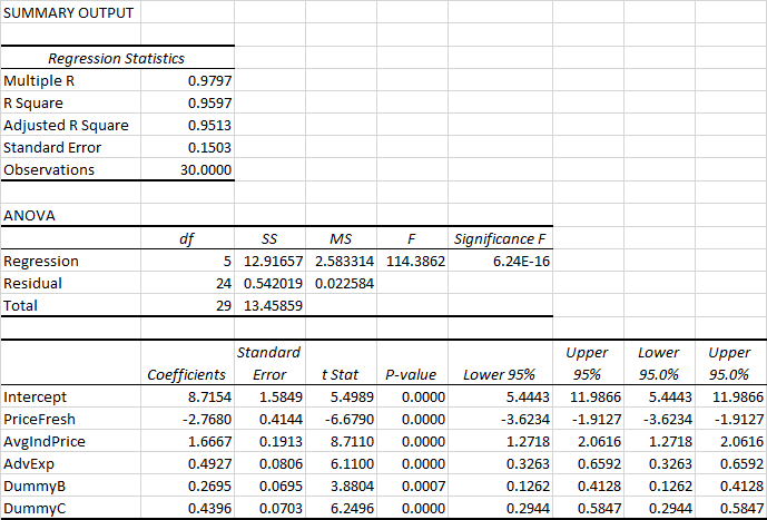
The Regression Equation is Demand_Fresh = 8.7154 + (-2.768*Price_Fresh) + (1.6667*Avg_Industry_Price) + (0.4927* Advertisement_Expense) + (0.2695*DB) + (0.4396*DC)

Step by step
Solved in 2 steps with 2 images


