Mech Velocity HW-4 2. Below is a position versus time graph of the motion of an object that has varying velocity. We will analyze this graph in detail around t = 2 s and x = 2 cm. a. In the interval from t=0 s to t = 6 s, does the object move with nearly constant velocity or with definitely varying velocity? Explain. 1 Table of x and t values between t = 1.5 s and t=2.5 s (to be plotted on graph at right) x (cm) t(s) 1.5 1.6 1.7 1.8 1.9 2.0 2.1 2.2 2.3 2.4 2.5 3.25 2.96 2.69 2.44 2.21 2.00 1.81 1.64 1.49 Position (centimeters) 1.36 1.25 Position (centimeters) 10 8 3.4 3.2 3.0 2.8 2.6 2.4 2.2 2.0 1.8 1.6 1.4 1.2 6 4 2 b. In the small box on the graph above is a portion of the graph that corresponds to the motion from t= 1.5 s to t=2.5 s.. Graph of position versus time for object moving along straight-line path The position and time coordinates for points in this small interval are given in the following table. Plot these points on the graph below to obtain an expanded view of this small interval. 1 1.4 2 3 4 Time (seconds) 1.6 Expanded graph of position versus time for object moving along straight-line path 5 H 1.8 2.0 Time (seconds) 2.2 6 24 2.6


Displacement, Velocity and Acceleration
In classical mechanics, kinematics deals with the motion of a particle. It deals only with the position, velocity, acceleration, and displacement of a particle. It has no concern about the source of motion.
Linear Displacement
The term "displacement" refers to when something shifts away from its original "location," and "linear" refers to a straight line. As a result, “Linear Displacement” can be described as the movement of an object in a straight line along a single axis, for example, from side to side or up and down. Non-contact sensors such as LVDTs and other linear location sensors can calculate linear displacement. Non-contact sensors such as LVDTs and other linear location sensors can calculate linear displacement. Linear displacement is usually measured in millimeters or inches and may be positive or negative.

To analyze the motion of a body from the position-time graph.
Given:
The graph: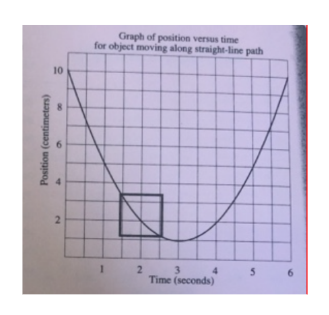
The data: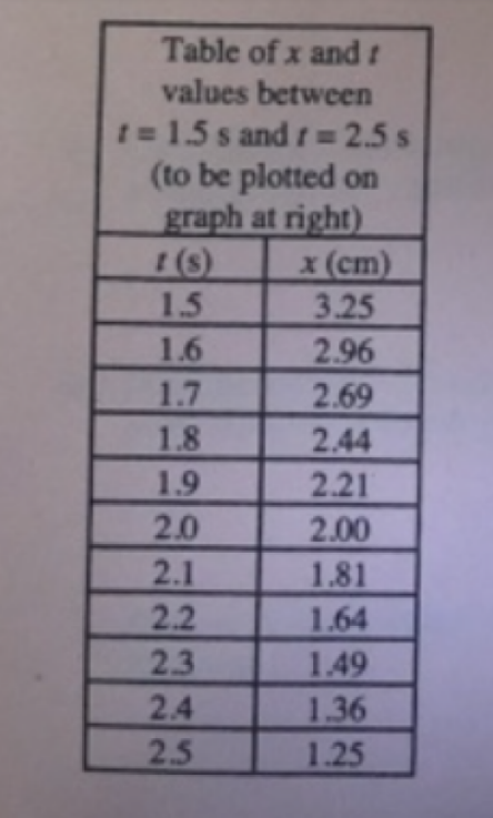
To obtain:
(a) Whether the object moves with constant velocity or with definitely varying velocity.
(b) To plot the graph for to

Trending now
This is a popular solution!

Step by step
Solved in 3 steps with 3 images


