= Normal Distribution with μ P(X> 1.28) = -1.28 -1 0 μ 0 and a = 1 1.28

MATLAB: An Introduction with Applications
6th Edition
ISBN:9781119256830
Author:Amos Gilat
Publisher:Amos Gilat
Chapter1: Starting With Matlab
Section: Chapter Questions
Problem 1P

Related questions
Question

Transcribed Image Text:### Normal Distribution Graphs
#### C. Normal Distribution with μ = 0 and σ = 1
- **Graph Description:**
- This graph shows a standard normal distribution curve, centered at μ = 0 with a standard deviation (σ) of 1.
- The x-axis is marked with values -3, -2, -1, 0, 1, 2, 3.
- Two vertical dashed lines are drawn at x = -1.28 and x = 1.28.
- The area beyond these points (shaded in blue) represents \( P(|X| > 1.28) \).
- The left tail and right tail regions are shaded to represent this probability.
- **Annotation:**
- \( 0.1003 \)
- A note below the graph states, "That is only the area of one tail."
#### D. Normal Distribution with μ = 0 and σ = 1
- **Graph Description:**
- Another standard normal distribution curve, with the same mean and standard deviation.
- Vertical dashed lines are at x = -1.64 and x = 1.64.
- Shaded areas in the tails indicate the probability \( P(|X| > 1.64) \).
These graphs are used to demonstrate the calculation of probabilities in a standard normal distribution, focusing on the areas in the tails beyond certain z-scores. The notes clarify the meaning of the shaded regions and the calculations involved.
Expert Solution
Step 1
(c)
Find the value of P(|x|>1.28) by using MINITAB.
The value of P(|x|>1.28) is obtained by using MINITAB.
- Choose Graph > Probability Distribution Plot choose View Probability> OK.
- From Distribution, choose ‘Normal’ distribution.
- Click the Shaded Area
- Choose X Value and Both Tail for the region of the curve to shade.
- Enter the data value as 1.28.
- Click OK.
Output obtained from MINITAB is given below:
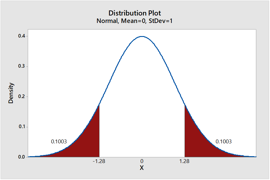
From the output, the value of P(|x|>1.28) is 0.2006 (=0.1003*2).

Step by step
Solved in 2 steps with 2 images

Recommended textbooks for you
MATLAB: An Introduction with Applications
Statistics
ISBN:
9781119256830
Author:
Amos Gilat
Publisher:
John Wiley & Sons Inc

Probability and Statistics for Engineering and th…
Statistics
ISBN:
9781305251809
Author:
Jay L. Devore
Publisher:
Cengage Learning

Statistics for The Behavioral Sciences (MindTap C…
Statistics
ISBN:
9781305504912
Author:
Frederick J Gravetter, Larry B. Wallnau
Publisher:
Cengage Learning
MATLAB: An Introduction with Applications
Statistics
ISBN:
9781119256830
Author:
Amos Gilat
Publisher:
John Wiley & Sons Inc
Probability and Statistics for Engineering and th…
Statistics
ISBN:
9781305251809
Author:
Jay L. Devore
Publisher:
Cengage Learning
Statistics for The Behavioral Sciences (MindTap C…
Statistics
ISBN:
9781305504912
Author:
Frederick J Gravetter, Larry B. Wallnau
Publisher:
Cengage Learning

Elementary Statistics: Picturing the World (7th E…
Statistics
ISBN:
9780134683416
Author:
Ron Larson, Betsy Farber
Publisher:
PEARSON

The Basic Practice of Statistics
Statistics
ISBN:
9781319042578
Author:
David S. Moore, William I. Notz, Michael A. Fligner
Publisher:
W. H. Freeman

Introduction to the Practice of Statistics
Statistics
ISBN:
9781319013387
Author:
David S. Moore, George P. McCabe, Bruce A. Craig
Publisher:
W. H. Freeman