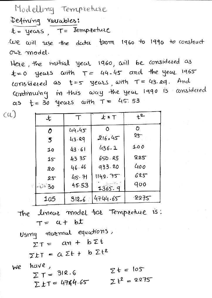
necpts developed in Precalculus to HIUdel aIi uctuul make a prediction. In this case we will model global warming The data: The following table summarizes the average yearly temperature (F")and carbon di emissions in parts per million (ppm) measured at Mauna Loa, Hawaii Year 1960 1965 1970 1975 1980 1985 1990 1995 2000 Temperature 44.45 43.29 43.61 320.0 325.7 45.71 45.53 345.9 354.2 43.35 46.66 47.53 45.86 CO2 316.9 331.1 338.7 360.6 369.4 Emissions Defining our variables: t = years after 1960, T = Temperature, and C = CO2 emissions. %3D We will use the data from the years 1960 and 1990 for our models. That is, for t = 0, T = 44.45 and C = 316.9 while for t = 30, T = 45.53 and C 354.2 Describe the Relationship 1) Modeling Temperature a) Use the data from 1960 and 1990 to find a linear function that model Temperature b) Use your linear function to predict the Temperature in 2005. Compa prediction with the actual Temperature in 2005. c) On graph paper, plot the entire set of temperature data from 1960 t On the same axis, plot your function from part (a) with at least 4 act the graph to give it some adequate scale. Discuss the similarities an the graph and the data. How well does your function approximate t

necpts developed in Precalculus to HIUdel aIi uctuul make a prediction. In this case we will model global warming The data: The following table summarizes the average yearly temperature (F")and carbon di emissions in parts per million (ppm) measured at Mauna Loa, Hawaii Year 1960 1965 1970 1975 1980 1985 1990 1995 2000 Temperature 44.45 43.29 43.61 320.0 325.7 45.71 45.53 345.9 354.2 43.35 46.66 47.53 45.86 CO2 316.9 331.1 338.7 360.6 369.4 Emissions Defining our variables: t = years after 1960, T = Temperature, and C = CO2 emissions. %3D We will use the data from the years 1960 and 1990 for our models. That is, for t = 0, T = 44.45 and C = 316.9 while for t = 30, T = 45.53 and C 354.2 Describe the Relationship 1) Modeling Temperature a) Use the data from 1960 and 1990 to find a linear function that model Temperature b) Use your linear function to predict the Temperature in 2005. Compa prediction with the actual Temperature in 2005. c) On graph paper, plot the entire set of temperature data from 1960 t On the same axis, plot your function from part (a) with at least 4 act the graph to give it some adequate scale. Discuss the similarities an the graph and the data. How well does your function approximate t

Name: Please help with number 1 portion a b and c pts developed in Precalcul
Uploaded: 2024-03-20T06:46:03.000Z
Channel: Bartleby
Description: Please help with number 1 portion a b and c pts developed in Precalculus to HIUdel an uctuurmake a prediction. In this case we will model global warmingThe data: The following table summarizes the average vearly temperature (F')and carbon dioxideemis

Calculus: Early Transcendentals

8th Edition

ISBN:9781285741550

Author:James Stewart

Publisher:James Stewart

Chapter1: Functions And Models

Section: Chapter Questions

Problem 1RCC: (a) What is a function? What are its domain and range? (b) What is the graph of a function? (c) How...

See similar textbooks

Related questions

Q: 3.57 Consider the experiment depicted by the Venn diagram, with the sample space S containing five…

A: As asked by you, I have answered the questions (C) and (D) only. Please find explanation below.…

Q: Number 14 parts d and e.

A: From the given Histogram, let us consider the following frequency table,

Q: Please upload a picture/PDF of your WORK and ANSWERS to following question: (-6, 2) (3, 2) Graph of…

A: c) The point of inflection is the value of x at which the derivative of the changes its concavity.

Q: Answer parts D, E & F

A: (d) From t table at 17 degrees of freedom, the area to the right of 1.740 is 0.050.…

Q: Consider the following results for independent samples taken from two populations. Sample 1 Sample 2…

A: The given data is as follows:Sample 1Sample 2

Q: Suppose George wins 26% of all staring contests. (a) What is the probability that George wins two…

A: a). Given that the probability of winning is 0.26. Multiply 0.26 by 0.26 to obtain the required…

Q: You may need to use the appropriate appendix table or technology to answer this question. A…

A: The probability that a potential customer makes a purchase is 0.10. Let the random variable X denote…

Q: n-1 b. It is a fact (proved by the 17th-century mathematicians Fermat and Pascal) that lim Use this…

Q: I need help on part d, part e, part f and part g

A: Given Level of significance ɑ=0.05 n=number of rows=5

Q: ssume that different groups of couples use a particular method of gender selection and each couple…

Q: ing Real World Relat Purpose: To use the concepts developed in Precalculus to model an actual make a…

A: Let t represent years after 1960. , C=CO2 emissions. Suppose the linear function that gives relation…

Q: k'( – 7) = b) k(x) = f(x)g(x) k'( – 7) = f(x) c) k(x) = g(x) 三 k'( – 7) =

Q: Let A= {a,,a2,a3} and B= {b,.b2.b3} be bases for a vector space V, and suppose b, = 5a, - 3a3, b2 =…

Q: One professor grades homework by randomly choosing 5 out of 12 homework problems to grade. (a) How…

A: Total no. Of homework problem = 12 Total no. Of problem selected = any 5

Q: c. Describe in words the meaning of the question "For what value of Tis f(T, 20) = -49?" Then answer…

A: Find your answer below

Q: (c) L[y] = y" + 2y' + 10y = 0 %3D (d) L[y] = x²y" + 5xy' + 4y = 0 %3D

Q: 7 0.25 10 0.10 12 0.25 14 0.35 16 0.25 18 0.05 0.65 10 0.35 (a) Construct a spreadsheet simulation…

Q: 4. Smith Electronics is a family-owned electronics repair business in Kansas City. The owner has…

A: We want to calculate the following mean , Variance and standard deviation

Q: (a) How many degrees does Earth turn in one hour? (b) How many degrees does Earth turn in one…

A: Given information:a. Earth turns 0.25° in one minute. b. It takes 2 minutes for moon to move…

Q: For the vectors u = (2, 0, 1) and v= (3, 1, 0), evaluate the following expressions. c. |u +3v| a. 2u…

Q: 6. Suppose the initial height from which a rubber ball drops is 100 in. The rebound heights to the…

Q: The use of the interval p + (z critical value) requires a large sample. For each of the following…

A: The confidence interval for sample proportion is given as: CI=p^±zcritp^1-p^n The required condition…

Q: H 4 Graph three different examples of a function that is not continuous (and therefore not…

Q: b) Determine if the following statements are logically equivalent. Ensure that you explain the steps…

A: (b) To Determine: Whether the following statements are equivalent or not: (i) ¬a→b∧¬b∨¬a∨¬b (ii)…

Q: ALZ 7.142 Studies on treating Alzheimer's disease. Alzheimer's disease is a progressive se of the…

A: Given information: The data represents the values of Alzheimer's disease.

Q: find part c

A: The provided information are: Population mean(μ)=2.2Population standard deviationσ=0.9

Q: c. Report the equation of the best-fit straight line, using weight as the predictor (x) and cost as…

A: Given data is weight(pounds)(x) cost(y) 12.3 17.08 18.8 23.84 20.4 26.82 16.5 19.85…

Q: Please complete all parts a, b, and c

A: Solution is given below

Q: Researchers are concerned about the rise in drinking behaviors among adolescents aged 13- 17 in a…

A: From the provided information, The research team estimates the prevalence of such behaviors is 17%…

Q: 10. A random sample of n - 4 individuals is selected from a population with µ = 35, and a treatment…

A: Solution : Given : n =4 μ = 35 M = 40.1 SS = 48 a. Difference…

Q: In 2011, a U.S. Census report determined that 71% of college students work. A researcher thinks this…

A: From the provided information, Sample size (n) = 110 From which 91 work. Sample proportion (p̂) =…

Concept explainers

Percentage

A percentage is a number indicated as a fraction of 100. It is a dimensionless number often expressed using the symbol %.

Algebraic Expressions

In mathematics, an algebraic expression consists of constant(s), variable(s), and mathematical operators. It is made up of terms.

Numbers

Numbers are some measures used for counting. They can be compared one with another to know its position in the number line and determine which one is greater or lesser than the other.

Subtraction

Before we begin to understand the subtraction of algebraic expressions, we need to list out a few things that form the basis of algebra.

Addition

Before we begin to understand the addition of algebraic expressions, we need to list out a few things that form the basis of algebra.

Topic Video

Question

Please help with number 1 portion a b and c

pts developed in Precalculus to HIUdel an uctuur
make a prediction. In this case we will model global warming
The data: The following table summarizes the average vearly temperature (F')and carbon dioxide
emissions in parts per million (ppm) measured at Mauna Loa, Hawail
Year
1960
1965
1970
1975
1980
1985
1990
1995
2000
2005
Temperature 44.45
43.29
43.61
43.35
46.66 45.71
45.53
47.53
45.86
46.23
CO2
316.9
320.0
325.7
331.1
338.7
345.9
354.2
360.6
369.4
379.7
Emissions
Defining our variables: t = years after 1960, T = Temperature, and C = CO2 emissions.
We will use the data from the years 1960 and 1990 for our models.
That is, for t = 0, T = 44.45 and C = 316.9 while for t = 30, T = 45.53 and C = 354.2
Describe the Relationship
1) Modeling Temperature
a) Use the data from 1960 and 1990 to find a linear function that models the
Temperature
b) Use your linear function to predict the Temperature in 2005. Compare your
prediction with the actual Temperature in 2005.
c) On graph paper, plot the entire set of temperature data from 1960 through 2005.
On the same axis, plot your function from part (a) with at least 4 actual points on
the graph to give it some adequate scale. Discuss the similarities and differences of
the graph and the data. How well does your function approximate the actual data?

Expert Solution

Step 1

Trending now

This is a popular solution!

Step by step

Solved in 3 steps with 3 images

SEE SOLUTION Check out a sample Q&A here

Knowledge Booster

$Algebraic Operations$

Learn more about

Need a deep-dive on the concept behind this application? Look no further. Learn more about this topic, calculus and related others by exploring similar questions and additional content below.