MPC-0.75 45-Degree Line 200 180 New AE Line 100 140 120 New Equilibrium 100 80 60 40 AE Line 20 o 20 40 0 80 100 120 140 180 180 200 REAL INCOME (Billins of dollars) In the first economy (with MPC = 0.5), the $20 billion increase in planned investment causes equilibrium income to increase by S second economy (with MPC = 0.75), the $20 billion increase in planned investment causes equilibrium income to increase by S | billion. In the billion. Therefore, a lower MPC is associated with a multiplier. Now, confirm your graphical analysis algebraically using the formula for the multiplier: Multiplier = AC For the first economy with an MPC of 0.5, the effect of the $20 billion increase in planned investment becomes the following: Change in Equilibrium Real Income = Change in Planned Expenditure × Multiplier Using the same method, the multiplier for the second economy is PLANNED EXPENDITURE (Billions of dollars) I| ||||
MPC-0.75 45-Degree Line 200 180 New AE Line 100 140 120 New Equilibrium 100 80 60 40 AE Line 20 o 20 40 0 80 100 120 140 180 180 200 REAL INCOME (Billins of dollars) In the first economy (with MPC = 0.5), the $20 billion increase in planned investment causes equilibrium income to increase by S second economy (with MPC = 0.75), the $20 billion increase in planned investment causes equilibrium income to increase by S | billion. In the billion. Therefore, a lower MPC is associated with a multiplier. Now, confirm your graphical analysis algebraically using the formula for the multiplier: Multiplier = AC For the first economy with an MPC of 0.5, the effect of the $20 billion increase in planned investment becomes the following: Change in Equilibrium Real Income = Change in Planned Expenditure × Multiplier Using the same method, the multiplier for the second economy is PLANNED EXPENDITURE (Billions of dollars) I| ||||

Chapter11: Managing Aggregate Demand: Fiscal Policy
Section11.A: Graphical Treatment Of Taxes And Fiscal Policy
Problem 3TY

Related questions
Question

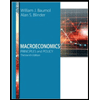
Transcribed Image Text:MPC=0.75
200
45-Degree Line
180
New AE Line
180
140
120
New Equilibrium
100
80
60
40
AE Line
20
20
40
60
80
100
120
140
160
180
200
REAL INCOME (Billions of dollars)
In the first economy (with MPC = 0.5), the $20 billion increase in planned investment causes equilibrium income to increase by $
billion. In the
second economy (with MPC = 0.75), the $20 billion increase in planned investment causes equilibrium income to increase by s
billion.
Therefore, a lower MPC is associated with a
multiplier.
Now, confirm your graphical analysis algebraically using the formula for the multiplier:
Multiplier = H MIC
For the first economy with an MPC of 0.5, the effect of the $20 billion increase in planned investment becomes the following:
Change in Equilibrium Real Income
Change in Planned Expenditure x Multiplier
%3D
Using the same method, the multiplier for the second economy is
PLANNED EXPENDITURE (Billions of dollars)
I| ||||

Transcribed Image Text:7. The multiplier and the MPC
Consider two closed economies that are identical except for their marginal propensity to consume (MPC). Each economy is currently in equilibrium with
real income and planned expenditure equal to $100 billion, as shown by the black points on the following two graphs. Neither economy has taxes that
change with income. The grey lines show the 45-degree line on each graph.
The first economy's MPC is 0.5. Therefore, its initial planned expenditure line has a slope of 0.5 and passes through the point (100o, 100).
The second economy's MPC is 0.75. Therefore, its initial planned expenditure line has a slope of 0.75 and passes through the point (100, 100).
Now, suppose there is an increase of $20 billion in planned investment in each economy.
Place a green line (triangle symbol) on each of the preceding graphs to indicate the new planned expenditure line for each economy. Then place a
black point (plus symbol) on each graph showing the new level of equilibrium income. (Hint: You can see the slope and vertical axis intercept of a line
on the graph by selecting it.)
MPC=0.5
45-Degree Line
200
180
New AE Line
160
140
120
New Equilibrium
100
80
60
AE Line
20
20
40
60
80
100 120
140
160
180
200
REAL INCOME (Billions of dollars)
PLANNED EXPE NDITURE (Billions of dollars)
Expert Solution
This question has been solved!
Explore an expertly crafted, step-by-step solution for a thorough understanding of key concepts.

This is a popular solution!

Trending now
This is a popular solution!

Step by step
Solved in 2 steps

Knowledge Booster


Learn more about
Need a deep-dive on the concept behind this application? Look no further. Learn more about this topic, economics and related others by exploring similar questions and additional content below.Recommended textbooks for you


Macroeconomics: Principles and Policy (MindTap Co…
Economics
ISBN:
9781305280601
Author:
William J. Baumol, Alan S. Blinder
Publisher:
Cengage Learning
