In order to improve the production time, the supervisor of assembly lines for a manufacturer of cellular phones has studied the time that it takes to assemble certain parts of a phone at various stations. She measures the time that it takes to assemble a specific part by 158 people at different shift on different days. The record of her study is organized and shown in the following table. Assume the normal distribution. (Due to the nature of this problem, do not use rounded intermediate values in your calculations-including answers submitted in WebAssign.)
In order to improve the production time, the supervisor of assembly lines for a manufacturer of cellular phones has studied the time that it takes to assemble certain parts of a phone at various stations. She measures the time that it takes to assemble a specific part by 158 people at different shift on different days. The record of her study is organized and shown in the following table. Assume the normal distribution. (Due to the nature of this problem, do not use rounded intermediate values in your calculations-including answers submitted in WebAssign.)
Elements Of Electromagnetics
7th Edition
ISBN:9780190698614
Author:Sadiku, Matthew N. O.
Publisher:Sadiku, Matthew N. O.
ChapterMA: Math Assessment
Section: Chapter Questions
Problem 1.1MA
Related questions
Question

Transcribed Image Text:In order to improve the production time, the supervisor of assembly lines for a manufacturer of cellular phones has studied the time that it takes to assemble certain parts of a phone at various stations. She measures the time that it takes to assemble a specific part by 158 people at different shifts
on different days. The record of her study is organized and shown in the following table. Assume the normal distribution. (Due to the nature of this problem, do not use rounded intermediate values in your calculations-including answers submitted in WebAssign.)
Time That it takes a person to Assemble the Part (minutes)
What is the mean (in minutes)?
x =
minutes
What is the standard deviation (in minutes)?
S=
157
Z =
4
5
6
7
8
9
10
minutes
What is the z value corresponding to 6 minutes?
X - X
6-
=*=*=.
S
Frequency
13
24
26
32
26
24
13
Expert Solution
This question has been solved!
Explore an expertly crafted, step-by-step solution for a thorough understanding of key concepts.
Step by step
Solved in 5 steps with 1 images

Follow-up Questions
Read through expert solutions to related follow-up questions below.
Follow-up Question

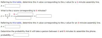
Transcribed Image Text:Referring to this table, determine the A value corresponding to the z value for a 6-minute-assembly line.
A =
What is the z score corresponding to 8 minutes?
8-
z =
X-X
S
=
Referring to this table, determine the A value corresponding to the z value for an 8-minute-assembly line.
A =
Determine the probability that it will take a person between 6 and 8 minutes to assemble the phone.
probability
=

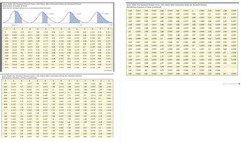
Transcribed Image Text:Areas Under the Standard Normal Curve-The Values Were Generated Using the Standard Normal
Distribution Function of Excel
Note that the standard normal curve is symmetrical about the mean.
z
0
0.01
0.02
0.03
0.04
0.05
0.06
0.07
0.08
0.09
0.1
0.11
0.12
1
0.95
0.96
0.97
0.98
0.99
1.01
1.02
1.03
1.04
1.05
Mean - 0
1.06
1.07
1.08
1.09
A
0.0000
0.0040
0.0080
0.0120
0.0160
0.0199
0.0239
0.0279
0.0319
0.0359
0.0398
0.0438
0.0478
A
0.3186
0.3212
0.3238
0.3264
0.3289
0.3315
0.3340
0.3365
0.3389
Z
0.3413
0.3438
0.3461
0.3485
0.3508
0.3531
0.3554
0.3577
0.3599
0.3621
0.13
0.14
0.15
0.16
0.17
0.18
0.19
0.2
0.21
0.22
0.23
0.24
0.25
1.12
1.13
1.14
1.15
1.16
1.17
A
z
0.0517
0.0557
0.26
0.27
0.28
0.29
0.0596
0.0636
0.0675 0.3
0.0714 0.31
0.0753 0.32
0.0793 0.33
0.0832 0.34
0.0871 0.35
0.0910
0.0948
0.0987
1.18
1.19
1.2
1.21
1.22
1.23
1.24
1.25
1.26
1.27
1.28
A
0.3643
0.3665
0.3686
0.3708
0.3729
0.3749
0.3770
0.3790
0.3810
0.36
0.3830
0.3849
0.3869
0.3888
0.3907
0.3925
0.3944
0.3962
0.3980
0.3997
0.37
0.38
z
1.29
1.3
1.31
1.32
1.33
1.34
1.35
A-03413
1.36
1.37
1.38
1.39
1.4
1.41
1.42
1.43
1.44
1.45
1.46
1.47
21.00
A
0.1026
0.1064
0.1103
Areas Under the Standard Normal Curve-The Values Were Generated Using the Standard Normal
Distribution Function of Excel (continued)
z
Z
0.91
0.92
0.93
1.1
1.11
0.94
0.1443
Z
0.44
0.1141
0.1179
0.1217
0.1255 0.45
0.1293 0.46
0.1331
0.47
0.1368 0.48
0.1406
0.49
0.5
0.51
0.1480
0.39
0.4
0.41
0.42
0.43
A
0.4015
0.4032
0.4049
0.4066
0.4082
0.4099
0.4115
0.4131
0.4147
0.4162
1.54
1.55
1.56
1.57
0.4177 1.58
0.4192 1.59
0.4207 1.6
0.4222 1.61
0.4236 1.62
0.4251 1.63
1.64
1.65
1.66
0.4265
0.4279
0.4292
z
1.48
1.49
1.5
1.51
1.52
A
0.1517
1.53
0.1554
0.1591
0.1628
0.1664
0,1700
0.1736
0.1772
0.1808
0.1844
0.1879
0.1915
0.1950
A
0.4306
0.4319
0.4332
0.4345
0.4357
0.4370
0.4382
0.4394
0.4406
0.4418
z
0.52
0.53
0.54
0.55
0.56
0.57
0.58
0.59
0.6
0.61
0.62
0.63
0.64
0.4429
0.4441
04452
0.4463
0.4474
0.4484
0.4495
0.4505
0.4515
z
1.67
1.68
1.69
1.7
1.71
1.72
1.73
1.74
1.75
1.76
1.77
1.78
1.79
1.8
A04772
1.81
1.82
1.83
1.84
1.85
z-2.00
Z
0.65
0.66
A
A
0.78
0.1985
0.2422
0.2019
0.2454 0.79
0.2054 0.67 0.2486 0.8
0.2088 0.68 0.2517
0.81
0.2123 0.69 0.2549 0.82
0.2157 0.7
0.2580 0.83
0.2190 0.71 0.2611 0.84
0.2224 0.72 0.2642 0.85
0.2257 0.73 0.2673 0.86
0.2291 0.74 0.2704 0.87
0.2324 0.75 0.2734 0.88
0.2357 0.76 0.2764
0.89
0.2389 0.77 0.2794 0.9
A
0.4525
0.4535
0.4545
0.4554
0.4564
0.4573
0.4582
0.4591
0.4599
0.4608
0.4616
0.4625
0.4633
0.4641
0.4649
0.4656
0.4664
0.4671
0.4678
z
1.86
1.87
1.88
1.89
1.9
1.91
1.92
1.93
1.94
1.95
1.96
1.97
1.98
1.99
2
Z
2.01
2.02
2.03
2.04
A-0.4987
A
z
0.4686 2.05
0.4693 2.06
0.4699
0.4706
2.08
0.4713 2.09
0.4719
2.1
0.4726 2.11
0.4732 2.12
0.4738 2.13
0.4744 2.14
0.4750 2.15
2.16
0.4756
0.4761 2.17
0.4767
2.18
0.4772 2.19
0.4778 2.2
0.4783 2.21
0.4788
0.4793
2.07
2.22
2.23
-3.00
A
0.2823
0.2852
0.2881
0.2910
0.2939
0.2967
0.2995
0.3023
0.3051
0.3078
0.3106
0.3133
0.3159
(continued)
A
0.4798
0.4803
0.4808
0.4812
0.4817
0.4821
0.4826
0.4830
0.4834
0.4838
0.4842
0.4846
0.4850
0.4854
0.4857
0.4861
0.4864
0.4868
0.4871
Areas Under the Standard Normal Curve-The Values Were Generated Using the Standard Normal
Distribution Function of Excel (continued)
2,24
2.26
2.27
2.28
0.4875 2.43 0.4925 2.62
0.4878 2.44 0.4927 2.63
0.4881 2.45 0.4929 2.64
0.4884 2.46 0.4931 2.65
0.4887 2.47
2.66
2.29 0.4890
2.48 0.4934 2.67
2.49
2.3 0.4893
0.4936
2.31 0.4896 2.5 0.4938 2.69
0.4898 2.51 0.4940 2.7
0.4901 2.52 0,4941 2.71
0.4904 2.53 0.4943 2.72
2.54 0.4945 2.73
0.4906
0.4909
2.55
0.4946 2.74
0.4911 2.56 0.4948 2.75
0.4913 2.57 0.4949 2.76
0.4916 2.58 0.4951 2.77
0.4918
0.4920 2.6 0.4953
0.4922 2.61 0.4955
2.78
2.79
2.25
2.32
2.33
2.34
2.35
2.36
2.37
2.38
2.39
2.4
2.41
2.42
2.59
0.4932
0.4952
2.68
2.8
0.4956
0.4957
0.4959
0.4960
0.4961
0.4962
0.4963
0.4964
0.4965
0.4966
0.4967 2.91
0.4968 2.92
0.4969 2.93
0.4970
2.94
0.4971 2.95
0.4972 2.96
0.4973 2.97
0.4974 2.98
0.4974 2.99
2.81 0.4975 3
0.4987 3.19
2.82 0.4976 3.01 0.4987 3.2
2.83 0.4977 3.02 0.4987 3.21
0.4977 3.03 0.4988 3.22
2.85 0.4978 3.04 0.4988 3.23
2.86 0.4979 3.05 0.4989
2.87
0.4979
3.06
2.88
3.07
2.89 0.4981 3.08
0.4981 3.09
0.4982
0.4980
2.84
2.9
0.4982
0.4983
3.1
3.11
3.12
3.13
0.4984
0.4984 3.14
0.4985 3.15
0.4985
0.4986 3.17
0.4986
3.16
0.4993 3.38
0.4993 3.39
0.4993 3.4
3.41
0.4994 3.42
0.4994 3.43
0.4994
3.25
3.44
0.4989 3.26 0.4994 3.45
0.4990 3.27
0.4990
3.18
0.4989
0.4990
0.4991
3.24
3.28
3.29
3.3
0.4991 3.31
0.4991 3.32
0.4992 3.33
0.4992 3.34
0.4992 3.35
0.4992 3.36
0.4993 3.37
0.4994
0.4995 3.46
0.4995 3.47
0.4995 3.48
0.4995 3.49
0.4995 3.5
0.4995 3.51
0.4996 3.52
0.4996 3.53
0.4996
0.4996
0.4996
***
***
3.9
0.4996
0.4997
0.4997
0.4997
0.4997
0.4997
0.4997
0.4997
0.4997
0.4997
0.4997
0.4998
0.4998
0.4998
0.4998
0.4998
c...
***
0.5000
End of document
Solution
Knowledge Booster
Learn more about
Need a deep-dive on the concept behind this application? Look no further. Learn more about this topic, mechanical-engineering and related others by exploring similar questions and additional content below.Recommended textbooks for you

Elements Of Electromagnetics
Mechanical Engineering
ISBN:
9780190698614
Author:
Sadiku, Matthew N. O.
Publisher:
Oxford University Press

Mechanics of Materials (10th Edition)
Mechanical Engineering
ISBN:
9780134319650
Author:
Russell C. Hibbeler
Publisher:
PEARSON

Thermodynamics: An Engineering Approach
Mechanical Engineering
ISBN:
9781259822674
Author:
Yunus A. Cengel Dr., Michael A. Boles
Publisher:
McGraw-Hill Education

Elements Of Electromagnetics
Mechanical Engineering
ISBN:
9780190698614
Author:
Sadiku, Matthew N. O.
Publisher:
Oxford University Press

Mechanics of Materials (10th Edition)
Mechanical Engineering
ISBN:
9780134319650
Author:
Russell C. Hibbeler
Publisher:
PEARSON

Thermodynamics: An Engineering Approach
Mechanical Engineering
ISBN:
9781259822674
Author:
Yunus A. Cengel Dr., Michael A. Boles
Publisher:
McGraw-Hill Education

Control Systems Engineering
Mechanical Engineering
ISBN:
9781118170519
Author:
Norman S. Nise
Publisher:
WILEY

Mechanics of Materials (MindTap Course List)
Mechanical Engineering
ISBN:
9781337093347
Author:
Barry J. Goodno, James M. Gere
Publisher:
Cengage Learning

Engineering Mechanics: Statics
Mechanical Engineering
ISBN:
9781118807330
Author:
James L. Meriam, L. G. Kraige, J. N. Bolton
Publisher:
WILEY