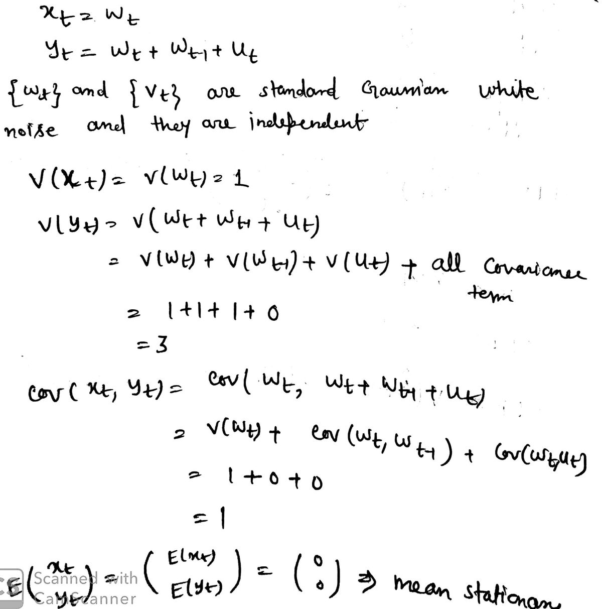
and they are independent
MATLAB: An Introduction with Applications
6th Edition
ISBN:9781119256830
Author:Amos Gilat
Publisher:Amos Gilat
Chapter1: Starting With Matlab
Section: Chapter Questions
Problem 1P
Related questions
Question
100%
![**Bivariate Time Series Model Analysis**
*Consider the following bivariate time series model:*
\[ x_t = w_t, \quad y_t = w_t + w_{t-1} + u_t, \]
*where \(\{w_t\}\) and \(\{u_t\}\) are standard (variance = 1) Gaussian white noise, and they are independent of each other.*
**Objective:**
Show that \((x_t, y_t)\) are jointly weakly stationary.
**Explanation:**
- \(x_t\) is equal to \(w_t\), which is a standard Gaussian white noise process with a mean of 0 and variance of 1.
- \(y_t\) is composed of three components: \(w_t\), the previous term \(w_{t-1}\), and another noise component \(u_t\). Each has a mean of 0 and variance of 1, and they contribute to the overall behavior of \(y_t\).
**To Show Joint Weak Stationarity:**
1. **Mean Constancy:**
- Verify that both \(x_t\) and \(y_t\) have constant means over time.
- Since each component is Gaussian white noise with a mean of 0, both \(x_t\) and \(y_t\) also have a mean of 0.
2. **Constant Variance:**
- The variance for \(x_t\) is simply the variance of \(w_t\), which is 1.
- The variance for \(y_t\) includes contributions from \(w_t\), \(w_{t-1}\), and \(u_t\), calculated as:
\[
\text{Var}(y_t) = \text{Var}(w_t) + \text{Var}(w_{t-1}) + \text{Var}(u_t) = 1 + 1 + 1 = 3
\]
3. **Covariance Consistency:**
- Calculate the covariance between \(x_t\) and \(y_t\).
- Since \(x_t\) only depends on \(w_t\), the covariance comes from the shared \(w_t\) component, resulting in:
\[
\text{Cov}(x_t, y_t) = \text{Cov}(w_t, w_t) = 1
\](/v2/_next/image?url=https%3A%2F%2Fcontent.bartleby.com%2Fqna-images%2Fquestion%2F551717d0-4b5a-4e64-aa61-7fb810951941%2F4a059003-6dbd-49a5-b164-6a5d9a565992%2F6t4g808_processed.png&w=3840&q=75)
Transcribed Image Text:**Bivariate Time Series Model Analysis**
*Consider the following bivariate time series model:*
\[ x_t = w_t, \quad y_t = w_t + w_{t-1} + u_t, \]
*where \(\{w_t\}\) and \(\{u_t\}\) are standard (variance = 1) Gaussian white noise, and they are independent of each other.*
**Objective:**
Show that \((x_t, y_t)\) are jointly weakly stationary.
**Explanation:**
- \(x_t\) is equal to \(w_t\), which is a standard Gaussian white noise process with a mean of 0 and variance of 1.
- \(y_t\) is composed of three components: \(w_t\), the previous term \(w_{t-1}\), and another noise component \(u_t\). Each has a mean of 0 and variance of 1, and they contribute to the overall behavior of \(y_t\).
**To Show Joint Weak Stationarity:**
1. **Mean Constancy:**
- Verify that both \(x_t\) and \(y_t\) have constant means over time.
- Since each component is Gaussian white noise with a mean of 0, both \(x_t\) and \(y_t\) also have a mean of 0.
2. **Constant Variance:**
- The variance for \(x_t\) is simply the variance of \(w_t\), which is 1.
- The variance for \(y_t\) includes contributions from \(w_t\), \(w_{t-1}\), and \(u_t\), calculated as:
\[
\text{Var}(y_t) = \text{Var}(w_t) + \text{Var}(w_{t-1}) + \text{Var}(u_t) = 1 + 1 + 1 = 3
\]
3. **Covariance Consistency:**
- Calculate the covariance between \(x_t\) and \(y_t\).
- Since \(x_t\) only depends on \(w_t\), the covariance comes from the shared \(w_t\) component, resulting in:
\[
\text{Cov}(x_t, y_t) = \text{Cov}(w_t, w_t) = 1
\
![Suppose \(\{y_t\}\) is given as in Problem 1, while \(\{x_t\}\) is instead given by the following signal-plus-noise model:
\[ x_t = t + y_t. \]
Find the **bivariate autocorrelation function** \(\rho_x(s, t)\) of \(\{x_t\}\) with justification. Hint: identify first which is the signal term (non-random) and which is the noise term (random, mean zero).](/v2/_next/image?url=https%3A%2F%2Fcontent.bartleby.com%2Fqna-images%2Fquestion%2F551717d0-4b5a-4e64-aa61-7fb810951941%2F4a059003-6dbd-49a5-b164-6a5d9a565992%2Fspdnmwh_processed.png&w=3840&q=75)
Transcribed Image Text:Suppose \(\{y_t\}\) is given as in Problem 1, while \(\{x_t\}\) is instead given by the following signal-plus-noise model:
\[ x_t = t + y_t. \]
Find the **bivariate autocorrelation function** \(\rho_x(s, t)\) of \(\{x_t\}\) with justification. Hint: identify first which is the signal term (non-random) and which is the noise term (random, mean zero).
Expert Solution
Step 1
*Answer:

Step by step
Solved in 2 steps with 2 images

Recommended textbooks for you

MATLAB: An Introduction with Applications
Statistics
ISBN:
9781119256830
Author:
Amos Gilat
Publisher:
John Wiley & Sons Inc

Probability and Statistics for Engineering and th…
Statistics
ISBN:
9781305251809
Author:
Jay L. Devore
Publisher:
Cengage Learning

Statistics for The Behavioral Sciences (MindTap C…
Statistics
ISBN:
9781305504912
Author:
Frederick J Gravetter, Larry B. Wallnau
Publisher:
Cengage Learning

MATLAB: An Introduction with Applications
Statistics
ISBN:
9781119256830
Author:
Amos Gilat
Publisher:
John Wiley & Sons Inc

Probability and Statistics for Engineering and th…
Statistics
ISBN:
9781305251809
Author:
Jay L. Devore
Publisher:
Cengage Learning

Statistics for The Behavioral Sciences (MindTap C…
Statistics
ISBN:
9781305504912
Author:
Frederick J Gravetter, Larry B. Wallnau
Publisher:
Cengage Learning

Elementary Statistics: Picturing the World (7th E…
Statistics
ISBN:
9780134683416
Author:
Ron Larson, Betsy Farber
Publisher:
PEARSON

The Basic Practice of Statistics
Statistics
ISBN:
9781319042578
Author:
David S. Moore, William I. Notz, Michael A. Fligner
Publisher:
W. H. Freeman

Introduction to the Practice of Statistics
Statistics
ISBN:
9781319013387
Author:
David S. Moore, George P. McCabe, Bruce A. Craig
Publisher:
W. H. Freeman