A simple random sample of size n is drawn. The sample mean, x, is found to be 17.7, and the sample standard deviation, s, is found to be 4.1. Click the icon to view the table of areas under the t-distribution. (a) Construct a 95% confidence interval about μ if the sample size, n, is 34. Lower bound: ; Upper bound: (Use ascending order. Round to two decimal places as needed.)
A simple random sample of size n is drawn. The sample mean, x, is found to be 17.7, and the sample standard deviation, s, is found to be 4.1. Click the icon to view the table of areas under the t-distribution. (a) Construct a 95% confidence interval about μ if the sample size, n, is 34. Lower bound: ; Upper bound: (Use ascending order. Round to two decimal places as needed.)
MATLAB: An Introduction with Applications
6th Edition
ISBN:9781119256830
Author:Amos Gilat
Publisher:Amos Gilat
Chapter1: Starting With Matlab
Section: Chapter Questions
Problem 1P
Related questions
Question

Transcribed Image Text:10/9/23, 10:40 AM
df
4
5
SOUHABHS 25%28 58332 85838523355558
0.05
1.963 3.078 6.314
0.816 1.061 1.386 1.886 2.920
0.765 0.978 1.250 1.638 2.353
0.741 0.941 1.190 1.533 2.132
0.727 0.920 1.156 1.476 2.015
0.906 1.134 1.440 1.943
1.119 1.415 1.895
1.108 1.397 1.860
6 0.718
7 0.711
0.896
0.889
12.706
4.303
3.182
2.776
2.571
2.447 2.612 3.143 3.707
2.365 2.517 2.998 3.499
2.306 2.449 2.896 3.355
2.262 2.398 2.821 3.250
2.228 2.359 2.764 3.169
2.201 2.328 2.718 3.106
2.179 2.303 2.681 3.055
2.160 2.282 2.650 3.012
2.145 2.264 2.624 2.977
2.131 2.249 2.602 2.947
2.120
2.235
2.110 2.224
2.101 2.214 2.552 2.878
2.205 2.539 2.861
2.197 2.528 2.845
2.921
2.583
2.567 2.898
2.831
2.819
2.807
2.492 2.797
ervoo
8 0.706
9 0.703 0.883 1.100 1.383 1.833
10 0.700
0.879 1.093
1.372 1.812
11 0.697 0.876 1.088 1.363 1.796
12 0.695 0.873 1.083 1.356 1.782
13 0.694 0.870 1.079 1.350 1.771
14 0.692 0.868 1.076 1.345 1.761
15 0.691 0.866 1.074 1.341 1.753
16 0.690
0.865
1.071 1.337 1.746
17 0.689 0.863 1.069 1.333 1.740
18 0.688
0.862 1.067 1.330 1.734
19 0.688
0.861 1.066 1.328 1.729 2.093
20 0.687 0.860 1.064 1.325 1.725 2.086
21 0.686 0.859 1.063 1.323 1.721 2.080
22 0.686 0.858 1.061 1.321 1.717 2.074
0.685 0.858 1.060 1.319 1.714 2.069
24 0.685 0.857 1.059 1.318 1.711 2.064
0.684 0.856 1.058 1.316 1.708 2.060
2.485 2.787
26 0.684 0.856 1.058 1.315 1.706
2.056
2.162 2.479
2.779
27 0.684 0.855 1.057 1.314 1.703 2.052 2.158 2.473 2.771
0.683 0.855 1.056 1.313 1.701 2.048 2.154 2.467 2.763
29 0.683 0.854 1.055 1.311 1.699 2.045 2.150 2.462 2.756
30 0.683 0.854 1.055 1.310 1.697 2.042
2.147 2.457
2.750
31 0.682 0.853 1.054 1.309 1.696 2.040
2.144 2.453
0.682 0.853 1.054 1.309 1.694 2.037 2.141 2.449
0.682 0.853 1.053 1.308 1.692 2.035 2.138 2.445 2.733
0.682 0.852 1.052 1.307 1.691 2.032
0.682 0.852 1.052 1.306 1.690 2.030
36 0.681
0.852
1.052 1.306 1.688 2.028 2.131 2.434 2.719
2.990
37 0.681 0.851 1.051 1.305 1.687
2.026 2.129 2.431
2.715 2.985
0.681 0.851 1.051 1.304 1.686 2.024 2.127 2.429 2.712 2.980
39 0.681 0.851 1.050 1.304 1.685 2.023 2.125
2.426 2.708
40 0.681 0.851 1.050
1.303 1.684
2.021
2.123
2.423
50 0.679 0.849 1.047 1.299 1.676 2.009 2.109
60 0.679 0.848 1.045 1.296 1.671 2.000 2.099
70 0.678 0.847 1.044 1.294 1.667 1.994 2.093 2.381 2.648
80 0.678 0.846 1.043 1.292 1.664 1.990 2.088 2.374 2.639
90 0.677 0.846 1.042 1.291 1.662 1.987 2.084 2.368 2.632
100 0.677 0.845
1.042 1.290 1.660 1.984 2.081 2.364 2.626
1000 0.675 0.842
1.037 1.282 1.646 1.962 2.056 2.330 2.581
Z
0.674 0.842 1.036 1.282 1.645 1.960 2.054 2.326 2.576
2.744
2.738
3.008
3.002
2.136 2.441 2.728
2.133 2.438 2.724
2.996
2.976
2.704 2.971
2.403
2.678
2.390
2.660
df
0.25
34
1 1.000 1.376
2
0.20
-Area in
right tail
0.25
0.15
0.20
0.15
0.10
0.10
Table VI
t-Distribution
Area in Right Tail
0.025
0.05
0.025
0.02
0.01
2.189 2.518
2.183 2.508
2.177 2.500
2.172
2.167
0.02
15.894 31.821
4.849 6.965
3.482 4.541 5.841
2.999 3.747 4.604
2.757 3.365 4.032
Area in Right Tail
Table of t-Distribution Areas
0.005 0.0025
0.0005
63.657 127.321 318.309 636.619
9.925 14.089 22.327 31.599
7.453 10.215 12.924
5.598
7.173
8.610
4.773
5.893
6.869
0.01
0.005
4.317
4.029
3.833
3.690
3.581
3.497
3.428
3.372
3.326
3.286
3.252
3.222
3.197
3.174
3.153
3.135
3.119
3.104
3.091
3.078
3.022
3.015
0.001
2.871
2.813
2.807
5.208
4.785
4.501
0.0025
4.297
4.144
4.025
3.930
3.852
3.787
3.733
3.686
3.646
3.610
3.067 3.435
3.057
3.421
3.047
3.038
3.030
3.579
3.552
3.527
3.505
3.485
3.467
3.450
3.408
3.396
3.385
3.375
3.365
3.356
3.348
3.340
3.333
3.326
3.319
2.937
2.915
2.899
2.887
3.195
2.878 3.183
3.313
3.307
3.261
3.232
3.211
3.174
3.098
3.090
0.001
5.959
5.408
5.041
4.781
4.587
4.437
4.318
4.221
4.140
4.073
4.015
3.965
3.922
3.883
3.850
3.819
3.792
3.768
3.745
3.725
3.707
3.690
3.674
3.659
3.646
3.633
3.622
3.611
3.601
3.591
3.582
3.574
3.566
3.558
3.551
3.496
3.460
3.435
3.416
3.402
3.390
3.300
3.291
0.0005
https://mylab.pearson.com/Student/PlayerHomework.aspx?homeworkId=661266309&questionId=49&flushed=false&cId=7616404&back-DoAssignments.aspx
1/1

Transcribed Image Text:A simple random sample of size n is drawn. The sample mean, x, is found to be 17.7, and the sample standard deviation, s, is found to be 4.1.
Click the icon to view the table of areas under the t-distribution.
(a) Construct a 95% confidence interval about µ if the sample size, n, is 34.
Lower bound:; Upper bound:
(Use ascending order. Round to two decimal places as needed.)
Expert Solution
This question has been solved!
Explore an expertly crafted, step-by-step solution for a thorough understanding of key concepts.
This is a popular solution!
Trending now
This is a popular solution!
Step by step
Solved in 3 steps with 3 images

Follow-up Questions
Read through expert solutions to related follow-up questions below.
Follow-up Question

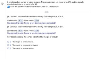
Transcribed Image Text:### Understanding Confidence Intervals and Margin of Error
**Sample Overview:**
A simple random sample of size \( n \) is drawn. The sample mean, \( \bar{x} \), is found to be 17.7, and the sample standard deviation, \( s \), is found to be 4.1.
**Confidence Interval Construction:**
- **(a)** For a sample size \( n = 34 \):
- **95% Confidence Interval:**
- Lower bound: 16.27
- Upper bound: 19.13
- Instruction: Use ascending order. Round to two decimal places as needed.
- **(b)** For a sample size \( n = 61 \):
- **95% Confidence Interval:**
- Lower bound: 16.65
- Upper bound: 18.75
- Instruction: Use ascending order. Round to two decimal places as needed.
**Effect of Sample Size on Margin of Error:**
How does increasing the sample size affect the margin of error, \( E \)?
- **Options:**
- A. The margin of error increases.
- B. The margin of error does not change.
- C. The margin of error decreases.
When the sample size increases, the margin of error typically decreases, making the confidence interval narrower. This indicates a more precise estimate of the population mean.
Solution
Follow-up Question

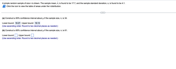
Transcribed Image Text:A simple random sample of size n is drawn. The sample mean, x, is found to be 17.7, and the sample standard deviation, s, is found to be 4.1.
Click the icon to view the table of areas under the t-distribution.
(a) Construct a 95% confidence interval about µ if the sample size, n, is 34.
Lower bound: 16.27; Upper bound: 19.13
(Use ascending order. Round to two decimal places as needed.)
(b) Construct a 95% confidence interval about μ if the sample size, n, is 61.
Lower bound:; Upper bound:
(Use ascending order. Round to two decimal places as needed.)
Solution
Recommended textbooks for you

MATLAB: An Introduction with Applications
Statistics
ISBN:
9781119256830
Author:
Amos Gilat
Publisher:
John Wiley & Sons Inc

Probability and Statistics for Engineering and th…
Statistics
ISBN:
9781305251809
Author:
Jay L. Devore
Publisher:
Cengage Learning

Statistics for The Behavioral Sciences (MindTap C…
Statistics
ISBN:
9781305504912
Author:
Frederick J Gravetter, Larry B. Wallnau
Publisher:
Cengage Learning

MATLAB: An Introduction with Applications
Statistics
ISBN:
9781119256830
Author:
Amos Gilat
Publisher:
John Wiley & Sons Inc

Probability and Statistics for Engineering and th…
Statistics
ISBN:
9781305251809
Author:
Jay L. Devore
Publisher:
Cengage Learning

Statistics for The Behavioral Sciences (MindTap C…
Statistics
ISBN:
9781305504912
Author:
Frederick J Gravetter, Larry B. Wallnau
Publisher:
Cengage Learning

Elementary Statistics: Picturing the World (7th E…
Statistics
ISBN:
9780134683416
Author:
Ron Larson, Betsy Farber
Publisher:
PEARSON

The Basic Practice of Statistics
Statistics
ISBN:
9781319042578
Author:
David S. Moore, William I. Notz, Michael A. Fligner
Publisher:
W. H. Freeman

Introduction to the Practice of Statistics
Statistics
ISBN:
9781319013387
Author:
David S. Moore, George P. McCabe, Bruce A. Craig
Publisher:
W. H. Freeman