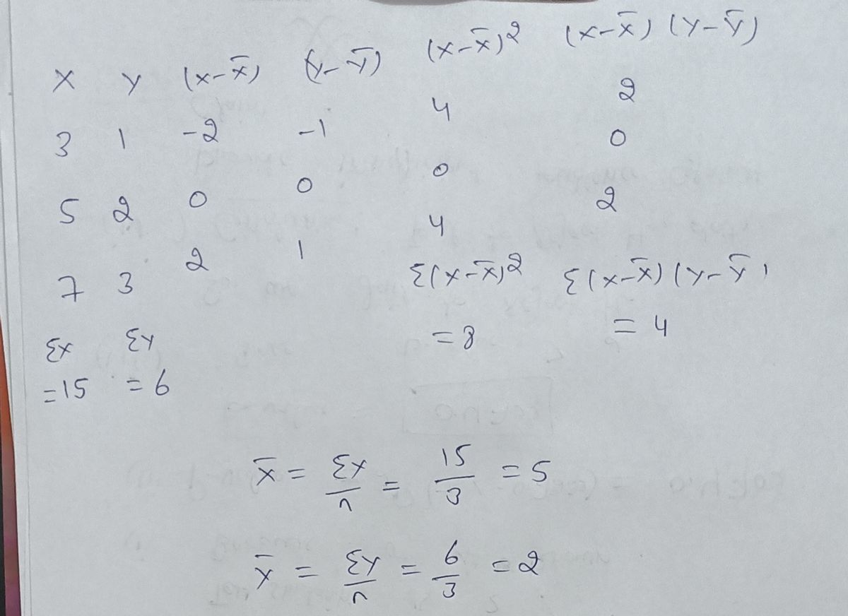
1. Suppose that you have the following data below: Y 1 3 2 5 7 Using either the linear algebra or summation notation formula, find B and B, the OLS estimates of the model
1. Suppose that you have the following data below: Y 1 3 2 5 7 Using either the linear algebra or summation notation formula, find B and B, the OLS estimates of the model

MATLAB: An Introduction with Applications
6th Edition
ISBN:9781119256830
Author:Amos Gilat
Publisher:Amos Gilat
Chapter1: Starting With Matlab
Section: Chapter Questions
Problem 1P

Related questions
Question
![1. Suppose that you have the following data below:
\[
\begin{array}{|c|c|}
\hline
Y & X \\
\hline
1 & 3 \\
2 & 5 \\
3 & 7 \\
\hline
\end{array}
\]
Using either the linear algebra or summation notation formula, find \(\widehat{\beta_0}\) and \(\widehat{\beta_1}\), the OLS estimates of the model.](/v2/_next/image?url=https%3A%2F%2Fcontent.bartleby.com%2Fqna-images%2Fquestion%2F375a2942-3f8b-4320-9caa-cc2588edb1a6%2Fe536b16a-9db0-412d-9bc2-8579272363f5%2F4rq024p_processed.png&w=3840&q=75)
Transcribed Image Text:1. Suppose that you have the following data below:
\[
\begin{array}{|c|c|}
\hline
Y & X \\
\hline
1 & 3 \\
2 & 5 \\
3 & 7 \\
\hline
\end{array}
\]
Using either the linear algebra or summation notation formula, find \(\widehat{\beta_0}\) and \(\widehat{\beta_1}\), the OLS estimates of the model.
![**Model Estimation and Regression Analysis**
To estimate the specified model of reorders, we use the equation:
\[ \text{Reorders}_i = \hat{\beta}_0 + \hat{\beta}_1 \cdot \text{Products}_i + \hat{\beta}_2 \cdot \text{Days}_i \]
where:
- \(\text{Reorders}_i\) is the number of reorders.
- \(\text{Products}_i\) is the number of ordered products.
- \(\text{Days}_i\) is the number of days since the last order.
The regression analysis, conducted in Excel, provides the following output:
### Regression Statistics
- **Multiple R**: 0.8373
- **R Square**: 0.7010
- **Adjusted R Square**: 0.6998
- **Standard Error**: 3.1710
- **Observations**: 500
### ANOVA Table
- **Regression**
- **df**: 2
- **SS**: 11717.33
- **MS**: 5858.67
- **Residual**
- **df**: 497
- **SS**: 4997.38
- **MS**: 10.06
- **Total**
- **df**: 499
- **SS**: 16714.71
- **F**: 582.66
- **Significance F**: 0.00
### Coefficients
1. **Intercept**
- Coefficient: 0.9778
- Standard Error: 0.3416
- t Stat: 2.8623
- P-value: 0.0044
- 95% Confidence Interval: [0.3066, 1.6489]
2. **Products**
- Coefficient: 0.6333
- Standard Error: 0.0188
- t Stat: 33.6482
- P-value: 0.0000
- 95% Confidence Interval: [0.5963, 0.6703]
3. **Days Since Prior Order**
- Coefficient: -0.0653
- Standard Error: 0.0133](/v2/_next/image?url=https%3A%2F%2Fcontent.bartleby.com%2Fqna-images%2Fquestion%2F375a2942-3f8b-4320-9caa-cc2588edb1a6%2Fe536b16a-9db0-412d-9bc2-8579272363f5%2Fvzadhu_processed.png&w=3840&q=75)
Transcribed Image Text:**Model Estimation and Regression Analysis**
To estimate the specified model of reorders, we use the equation:
\[ \text{Reorders}_i = \hat{\beta}_0 + \hat{\beta}_1 \cdot \text{Products}_i + \hat{\beta}_2 \cdot \text{Days}_i \]
where:
- \(\text{Reorders}_i\) is the number of reorders.
- \(\text{Products}_i\) is the number of ordered products.
- \(\text{Days}_i\) is the number of days since the last order.
The regression analysis, conducted in Excel, provides the following output:
### Regression Statistics
- **Multiple R**: 0.8373
- **R Square**: 0.7010
- **Adjusted R Square**: 0.6998
- **Standard Error**: 3.1710
- **Observations**: 500
### ANOVA Table
- **Regression**
- **df**: 2
- **SS**: 11717.33
- **MS**: 5858.67
- **Residual**
- **df**: 497
- **SS**: 4997.38
- **MS**: 10.06
- **Total**
- **df**: 499
- **SS**: 16714.71
- **F**: 582.66
- **Significance F**: 0.00
### Coefficients
1. **Intercept**
- Coefficient: 0.9778
- Standard Error: 0.3416
- t Stat: 2.8623
- P-value: 0.0044
- 95% Confidence Interval: [0.3066, 1.6489]
2. **Products**
- Coefficient: 0.6333
- Standard Error: 0.0188
- t Stat: 33.6482
- P-value: 0.0000
- 95% Confidence Interval: [0.5963, 0.6703]
3. **Days Since Prior Order**
- Coefficient: -0.0653
- Standard Error: 0.0133
Expert Solution
Step 1
Solution
As per guidelines we answer the only first question

Step by step
Solved in 2 steps with 2 images

Recommended textbooks for you
MATLAB: An Introduction with Applications
Statistics
ISBN:
9781119256830
Author:
Amos Gilat
Publisher:
John Wiley & Sons Inc

Probability and Statistics for Engineering and th…
Statistics
ISBN:
9781305251809
Author:
Jay L. Devore
Publisher:
Cengage Learning

Statistics for The Behavioral Sciences (MindTap C…
Statistics
ISBN:
9781305504912
Author:
Frederick J Gravetter, Larry B. Wallnau
Publisher:
Cengage Learning
MATLAB: An Introduction with Applications
Statistics
ISBN:
9781119256830
Author:
Amos Gilat
Publisher:
John Wiley & Sons Inc
Probability and Statistics for Engineering and th…
Statistics
ISBN:
9781305251809
Author:
Jay L. Devore
Publisher:
Cengage Learning
Statistics for The Behavioral Sciences (MindTap C…
Statistics
ISBN:
9781305504912
Author:
Frederick J Gravetter, Larry B. Wallnau
Publisher:
Cengage Learning

Elementary Statistics: Picturing the World (7th E…
Statistics
ISBN:
9780134683416
Author:
Ron Larson, Betsy Farber
Publisher:
PEARSON

The Basic Practice of Statistics
Statistics
ISBN:
9781319042578
Author:
David S. Moore, William I. Notz, Michael A. Fligner
Publisher:
W. H. Freeman

Introduction to the Practice of Statistics
Statistics
ISBN:
9781319013387
Author:
David S. Moore, George P. McCabe, Bruce A. Craig
Publisher:
W. H. Freeman