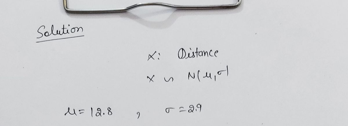
1. Draw a picture of the density curve with the mean labeled and shaded area representing the probability of a skate distance of 10 miles or more. Then, take a picture of your hand drawn sketch. 2. Use the Standard Normal Table to calculate the probability that a randomly selected Sunday skate will have a distance of 10 miles or more. Show all calculations needed to find this probability. 3. Use the Standard Normal Table to calculate the probability that that a randomly selected Sunday skate will have a distance between 9.9 and 12.8 miles. Show all calculations needed to find this probability. 4. Draw a picture of the density curve with the mean labeled and shaded area representing the probability of a skate distance that is in the shortest 1.5% (bottom 1.5%) or longest 2.5% (top 2.5%). Then, take a picture of the sketch.
1. Draw a picture of the density curve with the mean labeled and shaded area representing the
2. Use the Standard Normal Table to calculate the probability that a randomly selected Sunday skate will have a distance of 10 miles or more. Show all calculations needed to find this probability.
3. Use the Standard Normal Table to calculate the probability that that a randomly selected Sunday skate will have a distance between 9.9 and 12.8 miles. Show all calculations needed to find this probability.
4. Draw a picture of the density curve with the mean labeled and shaded area representing the probability of a skate distance that is in the shortest 1.5% (bottom 1.5%) or longest 2.5% (top 2.5%). Then, take a picture of the sketch.

We can solve only three subparts

Step by step
Solved in 2 steps with 2 images


