
Videos
a.
Explain the relationship between speed and density.
a.
Explanation of Solution
Given info:
The data related to the speed and density of traffic at the same location of a city at 10 different times within a span of 3 months.
Calculation:
Software procedure:
Step by step procedure to draw scatterplot using MINITAB software is given as,
- Choose Graph > Scatterplot.
- Choose Simple, and then click OK.
- In Y-variables, enter the column of Speed.
- In X-variables enter the column of Density.
- Click OK.
Output using MINITAB software is given as,
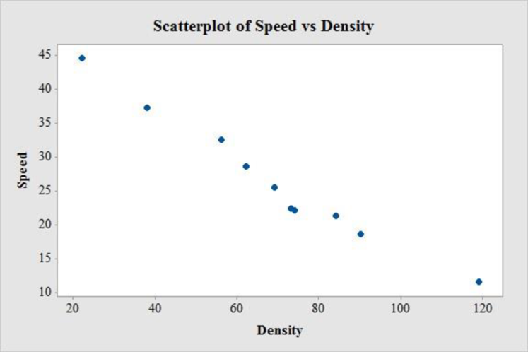
The relation between speed and density is strong, negative and linear. Thus, the association between speed and density is associated with lower speeds.
b.
Obtain a linear model to predict speed from density and comment on the appropriateness of the model.
b.
Answer to Problem 4E
The regression equation of linear model is
Explanation of Solution
Calculation:
Linear regression model:
A linear regression model is given as
Regression
Software procedure:
Step by step procedure to get the output using MINITAB software is given as,
- Choose Stat > Regression > Regression > Fit Regression Model.
- Under Responses, enter the column of Speed.
- Under predictors, enter the columns of Density.
- Click OK.
Output using MINITAB software is given below:
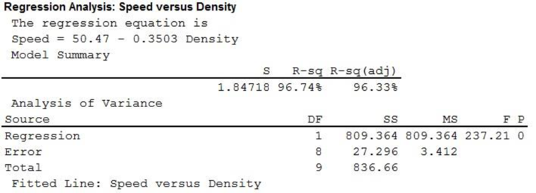
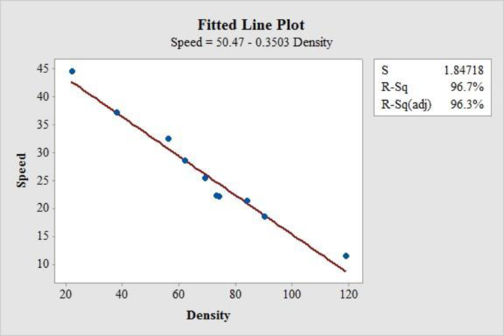
Thus, the regression equation of linear model is
The fitted scatterplot of re-expressed data exhibits a linear pattern. Thus, there is a strong and negative linear association between speed and density of traffic.
The coefficient of determination (
In the given output,
Thus, the 96.7% of the variability in speed is explained by density using linear regression model.
The conditions for a residual plot that is well fitted for the data are,
- There should not any bend, which would violate the straight line condition.
- There must not any outlier.
- There should not any change in the spread of the residuals from one part to another part of the plot.
Residual plot:
Software procedure:
Step by step procedure to get the output using MINITAB software is given as,
- Choose Stat > Regression > Regression > Fit Regression Model.
- Under Responses, enter the column of Speed.
- Under Continuous predictors, enter the columns of Density.
- In Graphs, under Residuals for plots choose Regular.
- Under Residuals plots choose Individuals plots and select box of Residuals versus fits.
- Click OK.
Output using MINITAB software is given below:
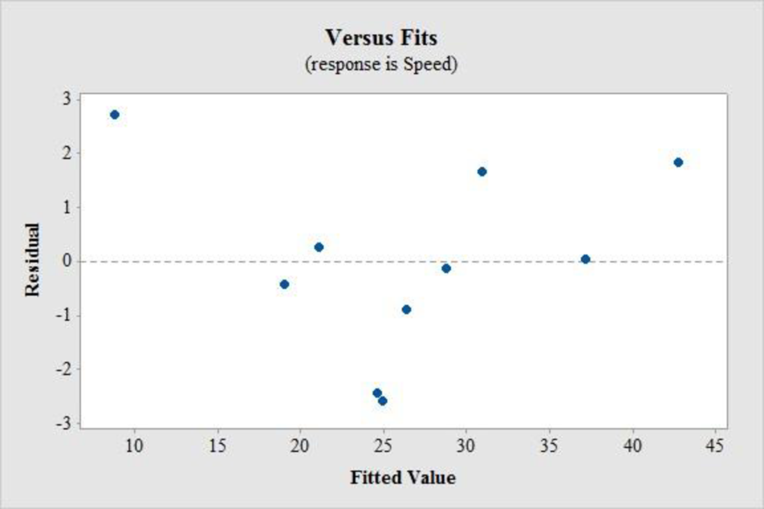
In residual plot, there is no bend or pattern, which can violate the straight line condition and there is no change in the spread of the residuals from one part to another part of the plot.
Thus, a linear model is appropriated.
c.
Find the residual of a traffic, having density and observed speed of 56 cars/mile and 32.5 mph, respectively.
Find the residual of another traffic, having density and observed speed of 20 cars/mile and 36.1 mph, respectively.
c.
Answer to Problem 4E
The residual of a traffic, having density and observed speed of 56 cars/mile and 32.5 mph, respectively is 1.65 mph and the residual of a traffic, having density and observed speed of 20 cars/mile and 36.1 mph, respectively is –7.36 mph.
Explanation of Solution
Calculation:
Assume x be the predictor variable and y be the response variable, of a
Residual:
The residual is defined as
If the observed value is less than predicted value then the residual will be negative and if the observed value is greater than predicted value then the residual will be positive.
From the previous part b. it is found that the regression equation of linear model is
The predicted speed of a traffic having density of 56 cars/mile is,
Thus, the predicted speed of a traffic having density of 56 cars/mile is 30.8532 mph.
It is known, that actual speed of a traffic having density of 56 cars/mile is 32.5 mph.
The value of the residual is,
Thus, the residual of a traffic, having density and observed speed of 56 cars/mile and 32.5 mph, respectively is 1.65 mph.
The predicted speed of a traffic having density of 20 cars/mile is,
Thus, the predicted speed of a traffic having density of 20 cars/mile is 43.46 mph.
It is known, that actual speed of a traffic having density of 20 cars/mile is 36.1 mph.
The value of the residual is,
Thus, the residual of a traffic, having density and observed speed of 20 cars/mile and 36.1 mph, respectively is –7.36 mph.
d.
Find the unusual residual.
d.
Answer to Problem 4E
Second residual is more unusual residual.
Explanation of Solution
From previous part c. it is found that residual of a traffic, having density and observed speed of 56 cars/mile and 32.5 mph, respectively is 1.65 mph and the residual of a traffic, having density and observed speed of 20 cars/mile and 36.1 mph, respectively is –7.36 mph.
Thus, it is clear that the second residual value is far away from the predicted value. Therefore, second residual is more unusual residual.
e.
Explain about slope and the
e.
Explanation of Solution
The new point
In another words, shallower slope and weaker correlation are closer to 0 as they are both started as negative quantity.
Thus, technically slope and correlation becomes higher.
f.
Predict the speed of traffic for a density of 200 cars/mile.
Explain whether the prediction is reasonable.
f.
Answer to Problem 4E
The predicted speed of a traffic having density of 200 cars/mile is –19.6 mph.
Explanation of Solution
Calculation:
The predicted speed of a traffic having density of 200 cars/mile is,
Thus, the predicted speed of a traffic having density of 200 cars/mile is –19.6 mph.
This result is not meaningful as the value of the speed comes as negative quantity, which cannot be possible. Moreover, the given car density of 200 cars/mile is far beyond from the observed values.
Thus, the prediction is not reasonable.
g.
Find the equation to predict the standardized speed from the standardized density if both the variables are standardized.
g.
Answer to Problem 4E
The equation to predict the standardized speed from the standardized density is
Explanation of Solution
Calculation:
z-score:
The z-score of a random variable x is defined as
Software Procedure:
Step by step procedure to obtain the correlation coefficient of the data using the MINITAB software:
- Choose Stat > Basic Statistics > Correlation.
- In Variables, enter the column of Speed and Density.
- Click OK in all dialogue boxes.
Output using the MINITAB software is given below:
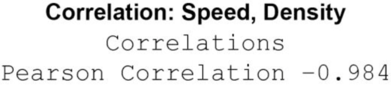
Thus, the correlation confident for speed and density is –0.984.
It is known that, the slope
Now, for the predictor variable x and response variable y also scarify the regression equation
Consider, the mean of the predictor variable x is
Subtract the equation
Using the formula
In this problem, as speed is the predictor variable (x) and density of traffic is response variable (y) with the correlation coefficient of
h.
Find the equation to predict the standardized density from the standardized speed if both the variables are standardized.
h.
Answer to Problem 4E
The equation to predict the standardized density from the standardized speed is
Explanation of Solution
Calculation:
From the previous part g. it is found that the correlation confident for speed and density is –0.984. In addition correlation is same regardless of the direction of prediction.
Consider, the mean of the predictor variable x is
Subtract the equation
Using the formula
In this problem, as density is the predictor variable (x) and speed of traffic is response variable (y) with the correlation coefficient of
Want to see more full solutions like this?
Chapter CR Solutions
STATS:DATA+MODELS(LL)-W/ACCESS>CUSTOM<


- Question: A company launches two different marketing campaigns to promote the same product in two different regions. After one month, the company collects the sales data (in units sold) from both regions to compare the effectiveness of the campaigns. The company wants to determine whether there is a significant difference in the mean sales between the two regions. Perform a two sample T-test You can provide your answer by inserting a text box and the answer must include: Null hypothesis, Alternative hypothesis, Show answer (output table/summary table), and Conclusion based on the P value. (2 points = 0.5 x 4 Answers) Each of these is worth 0.5 points. However, showing the calculation is must. If calculation is missing, the whole answer won't get any credit.arrow_forwardBinomial Prob. Question: A new teaching method claims to improve student engagement. A survey reveals that 60% of students find this method engaging. If 15 students are randomly selected, what is the probability that: a) Exactly 9 students find the method engaging?b) At least 7 students find the method engaging? (2 points = 1 x 2 answers) Provide answers in the yellow cellsarrow_forwardIn a survey of 2273 adults, 739 say they believe in UFOS. Construct a 95% confidence interval for the population proportion of adults who believe in UFOs. A 95% confidence interval for the population proportion is ( ☐, ☐ ). (Round to three decimal places as needed.)arrow_forward
- Find the minimum sample size n needed to estimate μ for the given values of c, σ, and E. C=0.98, σ 6.7, and E = 2 Assume that a preliminary sample has at least 30 members. n = (Round up to the nearest whole number.)arrow_forwardIn a survey of 2193 adults in a recent year, 1233 say they have made a New Year's resolution. Construct 90% and 95% confidence intervals for the population proportion. Interpret the results and compare the widths of the confidence intervals. The 90% confidence interval for the population proportion p is (Round to three decimal places as needed.) J.D) .arrow_forwardLet p be the population proportion for the following condition. Find the point estimates for p and q. In a survey of 1143 adults from country A, 317 said that they were not confident that the food they eat in country A is safe. The point estimate for p, p, is (Round to three decimal places as needed.) ...arrow_forward
- (c) Because logistic regression predicts probabilities of outcomes, observations used to build a logistic regression model need not be independent. A. false: all observations must be independent B. true C. false: only observations with the same outcome need to be independent I ANSWERED: A. false: all observations must be independent. (This was marked wrong but I have no idea why. Isn't this a basic assumption of logistic regression)arrow_forwardBusiness discussarrow_forwardSpam filters are built on principles similar to those used in logistic regression. We fit a probability that each message is spam or not spam. We have several variables for each email. Here are a few: to_multiple=1 if there are multiple recipients, winner=1 if the word 'winner' appears in the subject line, format=1 if the email is poorly formatted, re_subj=1 if "re" appears in the subject line. A logistic model was fit to a dataset with the following output: Estimate SE Z Pr(>|Z|) (Intercept) -0.8161 0.086 -9.4895 0 to_multiple -2.5651 0.3052 -8.4047 0 winner 1.5801 0.3156 5.0067 0 format -0.1528 0.1136 -1.3451 0.1786 re_subj -2.8401 0.363 -7.824 0 (a) Write down the model using the coefficients from the model fit.log_odds(spam) = -0.8161 + -2.5651 + to_multiple + 1.5801 winner + -0.1528 format + -2.8401 re_subj(b) Suppose we have an observation where to_multiple=0, winner=1, format=0, and re_subj=0. What is the predicted probability that this message is spam?…arrow_forward
- Consider an event X comprised of three outcomes whose probabilities are 9/18, 1/18,and 6/18. Compute the probability of the complement of the event. Question content area bottom Part 1 A.1/2 B.2/18 C.16/18 D.16/3arrow_forwardJohn and Mike were offered mints. What is the probability that at least John or Mike would respond favorably? (Hint: Use the classical definition.) Question content area bottom Part 1 A.1/2 B.3/4 C.1/8 D.3/8arrow_forwardThe details of the clock sales at a supermarket for the past 6 weeks are shown in the table below. The time series appears to be relatively stable, without trend, seasonal, or cyclical effects. The simple moving average value of k is set at 2. What is the simple moving average root mean square error? Round to two decimal places. Week Units sold 1 88 2 44 3 54 4 65 5 72 6 85 Question content area bottom Part 1 A. 207.13 B. 20.12 C. 14.39 D. 0.21arrow_forward
 MATLAB: An Introduction with ApplicationsStatisticsISBN:9781119256830Author:Amos GilatPublisher:John Wiley & Sons Inc
 Probability and Statistics for Engineering and th...StatisticsISBN:9781305251809Author:Jay L. DevorePublisher:Cengage Learning
 Statistics for The Behavioral Sciences (MindTap C...StatisticsISBN:9781305504912Author:Frederick J Gravetter, Larry B. WallnauPublisher:Cengage Learning
 Elementary Statistics: Picturing the World (7th E...StatisticsISBN:9780134683416Author:Ron Larson, Betsy FarberPublisher:PEARSON
 The Basic Practice of StatisticsStatisticsISBN:9781319042578Author:David S. Moore, William I. Notz, Michael A. FlignerPublisher:W. H. Freeman
 Introduction to the Practice of StatisticsStatisticsISBN:9781319013387Author:David S. Moore, George P. McCabe, Bruce A. CraigPublisher:W. H. Freeman