Videos
a.
Explain the relationship between speed and density.
a.
Explanation of Solution
Given info:
The data related to the speed and density of traffic at the same location of a city at 10 different times within a span of 3 months.
Calculation:
Software procedure:
Step by step procedure to draw scatterplot using MINITAB software is given as,
- Choose Graph > Scatterplot.
- Choose Simple, and then click OK.
- In Y-variables, enter the column of Speed.
- In X-variables enter the column of Density.
- Click OK.
Output using MINITAB software is given as,
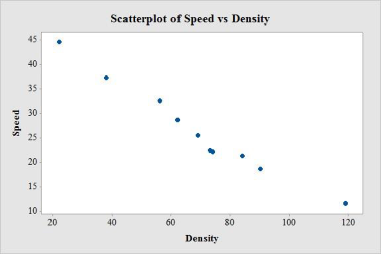
The relation between speed and density is strong, negative and linear. Thus, the association between speed and density is associated with lower speeds.
b.
Obtain a linear model to predict speed from density and comment on the appropriateness of the model.
b.
Answer to Problem 4E
The regression equation of linear model is
Explanation of Solution
Calculation:
Linear regression model:
A linear regression model is given as
Regression
Software procedure:
Step by step procedure to get the output using MINITAB software is given as,
- Choose Stat > Regression > Regression > Fit Regression Model.
- Under Responses, enter the column of Speed.
- Under predictors, enter the columns of Density.
- Click OK.
Output using MINITAB software is given below:
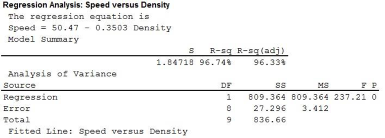
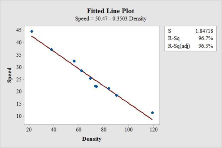
Thus, the regression equation of linear model is
The fitted scatterplot of re-expressed data exhibits a linear pattern. Thus, there is a strong and negative linear association between speed and density of traffic.
The coefficient of determination (
In the given output,
Thus, the 96.7% of the variability in speed is explained by density using linear regression model.
The conditions for a residual plot that is well fitted for the data are,
- There should not any bend, which would violate the straight line condition.
- There must not any outlier.
- There should not any change in the spread of the residuals from one part to another part of the plot.
Residual plot:
Software procedure:
Step by step procedure to get the output using MINITAB software is given as,
- Choose Stat > Regression > Regression > Fit Regression Model.
- Under Responses, enter the column of Speed.
- Under Continuous predictors, enter the columns of Density.
- In Graphs, under Residuals for plots choose Regular.
- Under Residuals plots choose Individuals plots and select box of Residuals versus fits.
- Click OK.
Output using MINITAB software is given below:
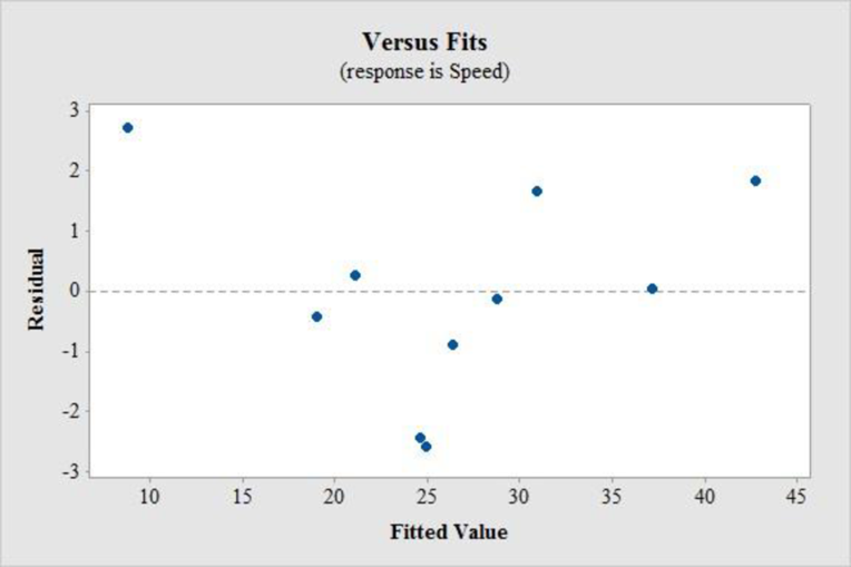
In residual plot, there is no bend or pattern, which can violate the straight line condition and there is no change in the spread of the residuals from one part to another part of the plot.
Thus, a linear model is appropriated.
c.
Find the residual of a traffic, having density and observed speed of 56 cars/mile and 32.5 mph, respectively.
Find the residual of another traffic, having density and observed speed of 20 cars/mile and 36.1 mph, respectively.
c.
Answer to Problem 4E
The residual of a traffic, having density and observed speed of 56 cars/mile and 32.5 mph, respectively is 1.65 mph and the residual of a traffic, having density and observed speed of 20 cars/mile and 36.1 mph, respectively is –7.36 mph.
Explanation of Solution
Calculation:
Assume x be the predictor variable and y be the response variable, of a
Residual:
The residual is defined as
If the observed value is less than predicted value then the residual will be negative and if the observed value is greater than predicted value then the residual will be positive.
From the previous part b. it is found that the regression equation of linear model is
The predicted speed of a traffic having density of 56 cars/mile is,
Thus, the predicted speed of a traffic having density of 56 cars/mile is 30.8532 mph.
It is known, that actual speed of a traffic having density of 56 cars/mile is 32.5 mph.
The value of the residual is,
Thus, the residual of a traffic, having density and observed speed of 56 cars/mile and 32.5 mph, respectively is 1.65 mph.
The predicted speed of a traffic having density of 20 cars/mile is,
Thus, the predicted speed of a traffic having density of 20 cars/mile is 43.46 mph.
It is known, that actual speed of a traffic having density of 20 cars/mile is 36.1 mph.
The value of the residual is,
Thus, the residual of a traffic, having density and observed speed of 20 cars/mile and 36.1 mph, respectively is –7.36 mph.
d.
Find the unusual residual.
d.
Answer to Problem 4E
Second residual is more unusual residual.
Explanation of Solution
From previous part c. it is found that residual of a traffic, having density and observed speed of 56 cars/mile and 32.5 mph, respectively is 1.65 mph and the residual of a traffic, having density and observed speed of 20 cars/mile and 36.1 mph, respectively is –7.36 mph.
Thus, it is clear that the second residual value is far away from the predicted value. Therefore, second residual is more unusual residual.
e.
Explain about slope and the
e.
Explanation of Solution
The new point
In another words, shallower slope and weaker correlation are closer to 0 as they are both started as negative quantity.
Thus, technically slope and correlation becomes higher.
f.
Predict the speed of traffic for a density of 200 cars/mile.
Explain whether the prediction is reasonable.
f.
Answer to Problem 4E
The predicted speed of a traffic having density of 200 cars/mile is –19.6 mph.
Explanation of Solution
Calculation:
The predicted speed of a traffic having density of 200 cars/mile is,
Thus, the predicted speed of a traffic having density of 200 cars/mile is –19.6 mph.
This result is not meaningful as the value of the speed comes as negative quantity, which cannot be possible. Moreover, the given car density of 200 cars/mile is far beyond from the observed values.
Thus, the prediction is not reasonable.
g.
Find the equation to predict the standardized speed from the standardized density if both the variables are standardized.
g.
Answer to Problem 4E
The equation to predict the standardized speed from the standardized density is
Explanation of Solution
Calculation:
z-score:
The z-score of a random variable x is defined as
Software Procedure:
Step by step procedure to obtain the correlation coefficient of the data using the MINITAB software:
- Choose Stat > Basic Statistics > Correlation.
- In Variables, enter the column of Speed and Density.
- Click OK in all dialogue boxes.
Output using the MINITAB software is given below:
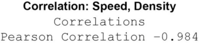
Thus, the correlation confident for speed and density is –0.984.
It is known that, the slope
Now, for the predictor variable x and response variable y also scarify the regression equation
Consider, the mean of the predictor variable x is
Subtract the equation
Using the formula
In this problem, as speed is the predictor variable (x) and density of traffic is response variable (y) with the correlation coefficient of
h.
Find the equation to predict the standardized density from the standardized speed if both the variables are standardized.
h.
Answer to Problem 4E
The equation to predict the standardized density from the standardized speed is
Explanation of Solution
Calculation:
From the previous part g. it is found that the correlation confident for speed and density is –0.984. In addition correlation is same regardless of the direction of prediction.
Consider, the mean of the predictor variable x is
Subtract the equation
Using the formula
In this problem, as density is the predictor variable (x) and speed of traffic is response variable (y) with the correlation coefficient of
Want to see more full solutions like this?
Chapter CR Solutions
Stats: Data and Models


- Analyze the residuals of a linear regression model and select the best response.Criteria is simple evaluation of possible indications of an exponential model vs. linear model) no, the residual plot does not show a curve yes, the residual plot does not show a curve yes, the residual plot shows a curve no, the residual plot shows a curve I selected: yes, the residual plot shows a curve and it is INCORRECT. Can u help me understand why?arrow_forwardYou have been hired as an intern to run analyses on the data and report the results back to Sarah; the five questions that Sarah needs you to address are given below. please do it step by step on excel Does there appear to be a positive or negative relationship between price and screen size? Use a scatter plot to examine the relationship. Determine and interpret the correlation coefficient between the two variables. In your interpretation, discuss the direction of the relationship (positive, negative, or zero relationship). Also discuss the strength of the relationship. Estimate the relationship between screen size and price using a simple linear regression model and interpret the estimated coefficients. (In your interpretation, tell the dollar amount by which price will change for each unit of increase in screen size). Include the manufacturer dummy variable (Samsung=1, 0 otherwise) and estimate the relationship between screen size, price and manufacturer dummy as a multiple…arrow_forwardHere is data with as the response variable. x y54.4 19.124.9 99.334.5 9.476.6 0.359.4 4.554.4 0.139.2 56.354 15.773.8 9-156.1 319.2Make a scatter plot of this data. Which point is an outlier? Enter as an ordered pair, e.g., (x,y). (x,y)= Find the regression equation for the data set without the outlier. Enter the equation of the form mx+b rounded to three decimal places. y_wo= Find the regression equation for the data set with the outlier. Enter the equation of the form mx+b rounded to three decimal places. y_w=arrow_forward
- You have been hired as an intern to run analyses on the data and report the results back to Sarah; the five questions that Sarah needs you to address are given below. please do it step by step Does there appear to be a positive or negative relationship between price and screen size? Use a scatter plot to examine the relationship. Determine and interpret the correlation coefficient between the two variables. In your interpretation, discuss the direction of the relationship (positive, negative, or zero relationship). Also discuss the strength of the relationship. Estimate the relationship between screen size and price using a simple linear regression model and interpret the estimated coefficients. (In your interpretation, tell the dollar amount by which price will change for each unit of increase in screen size). Include the manufacturer dummy variable (Samsung=1, 0 otherwise) and estimate the relationship between screen size, price and manufacturer dummy as a multiple linear…arrow_forwardExercises: Find all the whole number solutions of the congruence equation. 1. 3x 8 mod 11 2. 2x+3= 8 mod 12 3. 3x+12= 7 mod 10 4. 4x+6= 5 mod 8 5. 5x+3= 8 mod 12arrow_forwardScenario Sales of products by color follow a peculiar, but predictable, pattern that determines how many units will sell in any given year. This pattern is shown below Product Color 1995 1996 1997 Red 28 42 21 1998 23 1999 29 2000 2001 2002 Unit Sales 2003 2004 15 8 4 2 1 2005 2006 discontinued Green 26 39 20 22 28 14 7 4 2 White 43 65 33 36 45 23 12 Brown 58 87 44 48 60 Yellow 37 56 28 31 Black 28 42 21 Orange 19 29 Purple Total 28 42 21 49 68 78 95 123 176 181 164 127 24 179 Questions A) Which color will sell the most units in 2007? B) Which color will sell the most units combined in the 2007 to 2009 period? Please show all your analysis, leave formulas in cells, and specify any assumptions you make.arrow_forward
- One hundred students were surveyed about their preference between dogs and cats. The following two-way table displays data for the sample of students who responded to the survey. Preference Male Female TOTAL Prefers dogs \[36\] \[20\] \[56\] Prefers cats \[10\] \[26\] \[36\] No preference \[2\] \[6\] \[8\] TOTAL \[48\] \[52\] \[100\] problem 1 Find the probability that a randomly selected student prefers dogs.Enter your answer as a fraction or decimal. \[P\left(\text{prefers dogs}\right)=\] Incorrect Check Hide explanation Preference Male Female TOTAL Prefers dogs \[\blueD{36}\] \[\blueD{20}\] \[\blueE{56}\] Prefers cats \[10\] \[26\] \[36\] No preference \[2\] \[6\] \[8\] TOTAL \[48\] \[52\] \[100\] There were \[\blueE{56}\] students in the sample who preferred dogs out of \[100\] total students.arrow_forwardBusiness discussarrow_forwardYou have been hired as an intern to run analyses on the data and report the results back to Sarah; the five questions that Sarah needs you to address are given below. Does there appear to be a positive or negative relationship between price and screen size? Use a scatter plot to examine the relationship. Determine and interpret the correlation coefficient between the two variables. In your interpretation, discuss the direction of the relationship (positive, negative, or zero relationship). Also discuss the strength of the relationship. Estimate the relationship between screen size and price using a simple linear regression model and interpret the estimated coefficients. (In your interpretation, tell the dollar amount by which price will change for each unit of increase in screen size). Include the manufacturer dummy variable (Samsung=1, 0 otherwise) and estimate the relationship between screen size, price and manufacturer dummy as a multiple linear regression model. Interpret the…arrow_forward
- Does there appear to be a positive or negative relationship between price and screen size? Use a scatter plot to examine the relationship. How to take snapshots: if you use a MacBook, press Command+ Shift+4 to take snapshots. If you are using Windows, use the Snipping Tool to take snapshots. Question 1: Determine and interpret the correlation coefficient between the two variables. In your interpretation, discuss the direction of the relationship (positive, negative, or zero relationship). Also discuss the strength of the relationship. Value of correlation coefficient: Direction of the relationship (positive, negative, or zero relationship): Strength of the relationship (strong/moderate/weak): Question 2: Estimate the relationship between screen size and price using a simple linear regression model and interpret the estimated coefficients. In your interpretation, tell the dollar amount by which price will change for each unit of increase in screen size. (The answer for the…arrow_forwardIn this problem, we consider a Brownian motion (W+) t≥0. We consider a stock model (St)t>0 given (under the measure P) by d.St 0.03 St dt + 0.2 St dwt, with So 2. We assume that the interest rate is r = 0.06. The purpose of this problem is to price an option on this stock (which we name cubic put). This option is European-type, with maturity 3 months (i.e. T = 0.25 years), and payoff given by F = (8-5)+ (a) Write the Stochastic Differential Equation satisfied by (St) under the risk-neutral measure Q. (You don't need to prove it, simply give the answer.) (b) Give the price of a regular European put on (St) with maturity 3 months and strike K = 2. (c) Let X = S. Find the Stochastic Differential Equation satisfied by the process (Xt) under the measure Q. (d) Find an explicit expression for X₁ = S3 under measure Q. (e) Using the results above, find the price of the cubic put option mentioned above. (f) Is the price in (e) the same as in question (b)? (Explain why.)arrow_forwardProblem 4. Margrabe formula and the Greeks (20 pts) In the homework, we determined the Margrabe formula for the price of an option allowing you to swap an x-stock for a y-stock at time T. For stocks with initial values xo, yo, common volatility σ and correlation p, the formula was given by Fo=yo (d+)-x0Þ(d_), where In (±² Ꭲ d+ õ√T and σ = σ√√√2(1 - p). дго (a) We want to determine a "Greek" for ỡ on the option: find a formula for θα (b) Is дго θα positive or negative? (c) We consider a situation in which the correlation p between the two stocks increases: what can you say about the price Fo? (d) Assume that yo< xo and p = 1. What is the price of the option?arrow_forward
 MATLAB: An Introduction with ApplicationsStatisticsISBN:9781119256830Author:Amos GilatPublisher:John Wiley & Sons Inc
 Probability and Statistics for Engineering and th...StatisticsISBN:9781305251809Author:Jay L. DevorePublisher:Cengage Learning
 Statistics for The Behavioral Sciences (MindTap C...StatisticsISBN:9781305504912Author:Frederick J Gravetter, Larry B. WallnauPublisher:Cengage Learning
 Elementary Statistics: Picturing the World (7th E...StatisticsISBN:9780134683416Author:Ron Larson, Betsy FarberPublisher:PEARSON
 The Basic Practice of StatisticsStatisticsISBN:9781319042578Author:David S. Moore, William I. Notz, Michael A. FlignerPublisher:W. H. Freeman
 Introduction to the Practice of StatisticsStatisticsISBN:9781319013387Author:David S. Moore, George P. McCabe, Bruce A. CraigPublisher:W. H. Freeman