
Videos
a.
Explain the relationship between speed and density.
a.
Explanation of Solution
Given info:
The data related to the speed and density of traffic at the same location of a city at 10 different times within a span of 3 months.
Calculation:
Software procedure:
Step by step procedure to draw scatterplot using MINITAB software is given as,
- Choose Graph > Scatterplot.
- Choose Simple, and then click OK.
- In Y-variables, enter the column of Speed.
- In X-variables enter the column of Density.
- Click OK.
Output using MINITAB software is given as,
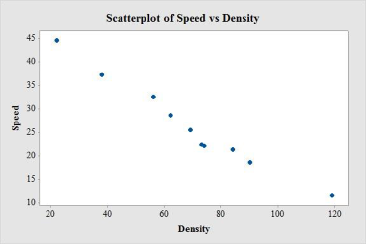
The relation between speed and density is strong, negative and linear. Thus, the association between speed and density is associated with lower speeds.
b.
Obtain a linear model to predict speed from density and comment on the appropriateness of the model.
b.
Answer to Problem 4E
The regression equation of linear model is
Explanation of Solution
Calculation:
Linear regression model:
A linear regression model is given as
Regression
Software procedure:
Step by step procedure to get the output using MINITAB software is given as,
- Choose Stat > Regression > Regression > Fit Regression Model.
- Under Responses, enter the column of Speed.
- Under predictors, enter the columns of Density.
- Click OK.
Output using MINITAB software is given below:
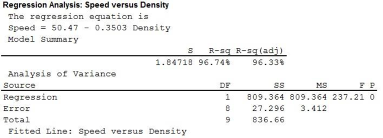
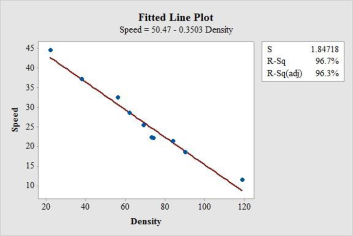
Thus, the regression equation of linear model is
The fitted scatterplot of re-expressed data exhibits a linear pattern. Thus, there is a strong and negative linear association between speed and density of traffic.
The coefficient of determination (
In the given output,
Thus, the 96.7% of the variability in speed is explained by density using linear regression model.
The conditions for a residual plot that is well fitted for the data are,
- There should not any bend, which would violate the straight line condition.
- There must not any outlier.
- There should not any change in the spread of the residuals from one part to another part of the plot.
Residual plot:
Software procedure:
Step by step procedure to get the output using MINITAB software is given as,
- Choose Stat > Regression > Regression > Fit Regression Model.
- Under Responses, enter the column of Speed.
- Under Continuous predictors, enter the columns of Density.
- In Graphs, under Residuals for plots choose Regular.
- Under Residuals plots choose Individuals plots and select box of Residuals versus fits.
- Click OK.
Output using MINITAB software is given below:
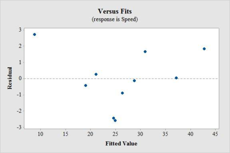
In residual plot, there is no bend or pattern, which can violate the straight line condition and there is no change in the spread of the residuals from one part to another part of the plot.
Thus, a linear model is appropriated.
c.
Find the residual of a traffic, having density and observed speed of 56 cars/mile and 32.5 mph, respectively.
Find the residual of another traffic, having density and observed speed of 20 cars/mile and 36.1 mph, respectively.
c.
Answer to Problem 4E
The residual of a traffic, having density and observed speed of 56 cars/mile and 32.5 mph, respectively is 1.65 mph and the residual of a traffic, having density and observed speed of 20 cars/mile and 36.1 mph, respectively is –7.36 mph.
Explanation of Solution
Calculation:
Assume x be the predictor variable and y be the response variable, of a
Residual:
The residual is defined as
If the observed value is less than predicted value then the residual will be negative and if the observed value is greater than predicted value then the residual will be positive.
From the previous part b. it is found that the regression equation of linear model is
The predicted speed of a traffic having density of 56 cars/mile is,
Thus, the predicted speed of a traffic having density of 56 cars/mile is 30.8532 mph.
It is known, that actual speed of a traffic having density of 56 cars/mile is 32.5 mph.
The value of the residual is,
Thus, the residual of a traffic, having density and observed speed of 56 cars/mile and 32.5 mph, respectively is 1.65 mph.
The predicted speed of a traffic having density of 20 cars/mile is,
Thus, the predicted speed of a traffic having density of 20 cars/mile is 43.46 mph.
It is known, that actual speed of a traffic having density of 20 cars/mile is 36.1 mph.
The value of the residual is,
Thus, the residual of a traffic, having density and observed speed of 20 cars/mile and 36.1 mph, respectively is –7.36 mph.
d.
Find the unusual residual.
d.
Answer to Problem 4E
Second residual is more unusual residual.
Explanation of Solution
From previous part c. it is found that residual of a traffic, having density and observed speed of 56 cars/mile and 32.5 mph, respectively is 1.65 mph and the residual of a traffic, having density and observed speed of 20 cars/mile and 36.1 mph, respectively is –7.36 mph.
Thus, it is clear that the second residual value is far away from the predicted value. Therefore, second residual is more unusual residual.
e.
Explain about slope and the
e.
Explanation of Solution
The new point
In another words, shallower slope and weaker correlation are closer to 0 as they are both started as negative quantity.
Thus, technically slope and correlation becomes higher.
f.
Predict the speed of traffic for a density of 200 cars/mile.
Explain whether the prediction is reasonable.
f.
Answer to Problem 4E
The predicted speed of a traffic having density of 200 cars/mile is –19.6 mph.
Explanation of Solution
Calculation:
The predicted speed of a traffic having density of 200 cars/mile is,
Thus, the predicted speed of a traffic having density of 200 cars/mile is –19.6 mph.
This result is not meaningful as the value of the speed comes as negative quantity, which cannot be possible. Moreover, the given car density of 200 cars/mile is far beyond from the observed values.
Thus, the prediction is not reasonable.
g.
Find the equation to predict the standardized speed from the standardized density if both the variables are standardized.
g.
Answer to Problem 4E
The equation to predict the standardized speed from the standardized density is
Explanation of Solution
Calculation:
z-score:
The z-score of a random variable x is defined as
Software Procedure:
Step by step procedure to obtain the correlation coefficient of the data using the MINITAB software:
- Choose Stat > Basic Statistics > Correlation.
- In Variables, enter the column of Speed and Density.
- Click OK in all dialogue boxes.
Output using the MINITAB software is given below:
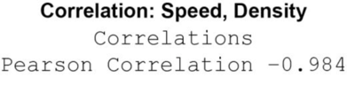
Thus, the correlation confident for speed and density is –0.984.
It is known that, the slope
Now, for the predictor variable x and response variable y also scarify the regression equation
Consider, the mean of the predictor variable x is
Subtract the equation
Using the formula
In this problem, as speed is the predictor variable (x) and density of traffic is response variable (y) with the correlation coefficient of
h.
Find the equation to predict the standardized density from the standardized speed if both the variables are standardized.
h.
Answer to Problem 4E
The equation to predict the standardized density from the standardized speed is
Explanation of Solution
Calculation:
From the previous part g. it is found that the correlation confident for speed and density is –0.984. In addition correlation is same regardless of the direction of prediction.
Consider, the mean of the predictor variable x is
Subtract the equation
Using the formula
In this problem, as density is the predictor variable (x) and speed of traffic is response variable (y) with the correlation coefficient of
Want to see more full solutions like this?
Chapter CR Solutions
Stats


- Harvard University California Institute of Technology Massachusetts Institute of Technology Stanford University Princeton University University of Cambridge University of Oxford University of California, Berkeley Imperial College London Yale University University of California, Los Angeles University of Chicago Johns Hopkins University Cornell University ETH Zurich University of Michigan University of Toronto Columbia University University of Pennsylvania Carnegie Mellon University University of Hong Kong University College London University of Washington Duke University Northwestern University University of Tokyo Georgia Institute of Technology Pohang University of Science and Technology University of California, Santa Barbara University of British Columbia University of North Carolina at Chapel Hill University of California, San Diego University of Illinois at Urbana-Champaign National University of Singapore McGill…arrow_forwardName Harvard University California Institute of Technology Massachusetts Institute of Technology Stanford University Princeton University University of Cambridge University of Oxford University of California, Berkeley Imperial College London Yale University University of California, Los Angeles University of Chicago Johns Hopkins University Cornell University ETH Zurich University of Michigan University of Toronto Columbia University University of Pennsylvania Carnegie Mellon University University of Hong Kong University College London University of Washington Duke University Northwestern University University of Tokyo Georgia Institute of Technology Pohang University of Science and Technology University of California, Santa Barbara University of British Columbia University of North Carolina at Chapel Hill University of California, San Diego University of Illinois at Urbana-Champaign National University of Singapore…arrow_forwardA company found that the daily sales revenue of its flagship product follows a normal distribution with a mean of $4500 and a standard deviation of $450. The company defines a "high-sales day" that is, any day with sales exceeding $4800. please provide a step by step on how to get the answers in excel Q: What percentage of days can the company expect to have "high-sales days" or sales greater than $4800? Q: What is the sales revenue threshold for the bottom 10% of days? (please note that 10% refers to the probability/area under bell curve towards the lower tail of bell curve) Provide answers in the yellow cellsarrow_forward
- Find the critical value for a left-tailed test using the F distribution with a 0.025, degrees of freedom in the numerator=12, and degrees of freedom in the denominator = 50. A portion of the table of critical values of the F-distribution is provided. Click the icon to view the partial table of critical values of the F-distribution. What is the critical value? (Round to two decimal places as needed.)arrow_forwardA retail store manager claims that the average daily sales of the store are $1,500. You aim to test whether the actual average daily sales differ significantly from this claimed value. You can provide your answer by inserting a text box and the answer must include: Null hypothesis, Alternative hypothesis, Show answer (output table/summary table), and Conclusion based on the P value. Showing the calculation is a must. If calculation is missing,so please provide a step by step on the answers Numerical answers in the yellow cellsarrow_forwardShow all workarrow_forward
 MATLAB: An Introduction with ApplicationsStatisticsISBN:9781119256830Author:Amos GilatPublisher:John Wiley & Sons Inc
 Probability and Statistics for Engineering and th...StatisticsISBN:9781305251809Author:Jay L. DevorePublisher:Cengage Learning
 Statistics for The Behavioral Sciences (MindTap C...StatisticsISBN:9781305504912Author:Frederick J Gravetter, Larry B. WallnauPublisher:Cengage Learning
 Elementary Statistics: Picturing the World (7th E...StatisticsISBN:9780134683416Author:Ron Larson, Betsy FarberPublisher:PEARSON
 The Basic Practice of StatisticsStatisticsISBN:9781319042578Author:David S. Moore, William I. Notz, Michael A. FlignerPublisher:W. H. Freeman
 Introduction to the Practice of StatisticsStatisticsISBN:9781319013387Author:David S. Moore, George P. McCabe, Bruce A. CraigPublisher:W. H. Freeman