
Concept explainers
Videos
Please provide the following information for Problems 11-22.
(a) What is the level of significance? State the null and alternate hypotheses.
(b)Check Requirements What sampling distribution will you use? Explain the rationale for your choice of sampling distribution. Compute the appropriate sampling distribution value of the sample test statistic.
(c) Find (or estimate) the P-value. Sketch the sampling distribution and show the area corresponding to the P- value.
(d) Based on your answers in parts (a) to (c), will you reject or fail to reject the null hypothesis? Are the data statistically significant at level ?
(e)Interpret your conclusion in the context of the application.
Note: For degrees of freedom d.f. not given in the Student's t table, use the closest d.f. that is smaller. In some situations, this choice of d.f. may increase the P-value by a small amount and therefore produce a slightly more “conservative" answer.
Ski Patrol: Avalanches Snow avalanches can be a real problem for travelers in the western United States and Canada. A very common type of avalanche is called the slab avalanche. These have been studied extensively by David McClung, a professor of civil engineering at the University of British Columbia. Slab avalanches studied in Canada have an average thickness of
A random sample of avalanches in spring gave the following thicknesses (in cm):
| 59 | 51 | 76 | 38 | 65 | 54 | 49 | 62 |
| 68 | 55 | 64 | 67 | 63 | 74 | 65 | 79 |
i. Use a calculator with
ii. Assume the slab thickness has an approximately
(i)
Whether the sample mean
Answer to Problem 19P
Solution: Yes, the sample mean
Explanation of Solution
To calculate the required statistics using the Minitab, follow the below instructions:
Step 1: Go to the Minitab software.
Step 2: Go to Stat > Basic statistics > Display Descriptive Statistics.
Step 3: Select ‘Thickness’ in variables.
Step 4: Click on OK.
The obtained statistics is:
Statistics
| Variable | N | N* | Mean | SE Mean | StDev | Minimum | Q1 | Median | Q3 | Maximum |
| Thickness | 16 | 0 | 61.81 | 2.66 | 10.65 | 38.00 | 54.25 | 63.50 | 67.75 | 79.00 |
From the Minitab output, the sample mean and sample standard deviation are approximately equals to
(ii)
(a)
The level of significance, null and alternative hypothesis.
Answer to Problem 19P
Solution: The level of significance is
Explanation of Solution
The level of significance is defined as the probability of rejecting the null hypothesis when it is true, it is denoted by
Null hypothesis
Alternative hypothesis
(b)
To find: The sampling distribution that should be used and compute the value of the sample test statistic.
Answer to Problem 19P
Solution: The student’s t distribution should be used. The sample test statistic is -1.96.
Explanation of Solution
Calculation:
We assume that x distribution is mound shape and symmetrical, because
Using
The sample test statistic t is
(c)
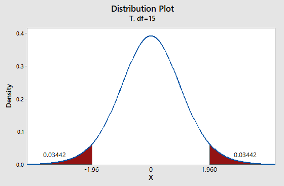
To find: The P-value of the test statistic and sketch the sampling distribution showing the area corresponding to the P-value.
Answer to Problem 19P
Solution: The P-value of the test statistic is 0.0688.
Explanation of Solution
Calculation:
We have t = -1.96
Using Table 4 from the Appendix to find the specified area:
Graph:
To draw the required graphs using the Minitab, follow the below instructions:
Step 1: Go to the Minitab software.
Step 2: Go to Graph > Probability distribution plot > View probability.
Step 3: Select ‘t’ and enter d.f = 15.
Step 4: Click on the Shaded area >X value.
Step 5: Enter X-value as -1.96 and select ‘Both Tail’.
Step 6: Click on OK.
The obtained distribution graph is:
(d)
Whether we reject or fail to reject the null hypothesis and whether the data is statistically significant for a level of significance of 0.01.
Answer to Problem 19P
Solution: The P-value
Explanation of Solution
The P-value of 0.0688 is greater than the level of significance (
) of 0.01. Therefore we don’t have enough evidence to reject the null hypothesis
(e)
The interpretation for the conclusion.
Answer to Problem 19P
Solution: There is not enough evidence to conclude that the mean slab thickness in the Vail region is different from that in Canada.
Explanation of Solution
The P-value of 0.0688 is greater than the level of significance (
) of 0.01. Therefore we don’t have enough evidence to reject the null hypothesis
Want to see more full solutions like this?
Chapter 9 Solutions
Bundle: Understanding Basic Statistics, Loose-leaf Version, 8th + WebAssign Printed Access Card, Single-Term


- Faye cuts the sandwich in two fair shares to her. What is the first half s1arrow_forwardQuestion 2. An American option on a stock has payoff given by F = f(St) when it is exercised at time t. We know that the function f is convex. A person claims that because of convexity, it is optimal to exercise at expiration T. Do you agree with them?arrow_forwardQuestion 4. We consider a CRR model with So == 5 and up and down factors u = 1.03 and d = 0.96. We consider the interest rate r = 4% (over one period). Is this a suitable CRR model? (Explain your answer.)arrow_forward
- Question 3. We want to price a put option with strike price K and expiration T. Two financial advisors estimate the parameters with two different statistical methods: they obtain the same return rate μ, the same volatility σ, but the first advisor has interest r₁ and the second advisor has interest rate r2 (r1>r2). They both use a CRR model with the same number of periods to price the option. Which advisor will get the larger price? (Explain your answer.)arrow_forwardQuestion 5. We consider a put option with strike price K and expiration T. This option is priced using a 1-period CRR model. We consider r > 0, and σ > 0 very large. What is the approximate price of the option? In other words, what is the limit of the price of the option as σ∞. (Briefly justify your answer.)arrow_forwardQuestion 6. You collect daily data for the stock of a company Z over the past 4 months (i.e. 80 days) and calculate the log-returns (yk)/(-1. You want to build a CRR model for the evolution of the stock. The expected value and standard deviation of the log-returns are y = 0.06 and Sy 0.1. The money market interest rate is r = 0.04. Determine the risk-neutral probability of the model.arrow_forward
- Several markets (Japan, Switzerland) introduced negative interest rates on their money market. In this problem, we will consider an annual interest rate r < 0. We consider a stock modeled by an N-period CRR model where each period is 1 year (At = 1) and the up and down factors are u and d. (a) We consider an American put option with strike price K and expiration T. Prove that if <0, the optimal strategy is to wait until expiration T to exercise.arrow_forwardWe consider an N-period CRR model where each period is 1 year (At = 1), the up factor is u = 0.1, the down factor is d = e−0.3 and r = 0. We remind you that in the CRR model, the stock price at time tn is modeled (under P) by Sta = So exp (μtn + σ√AtZn), where (Zn) is a simple symmetric random walk. (a) Find the parameters μ and σ for the CRR model described above. (b) Find P Ste So 55/50 € > 1). StN (c) Find lim P 804-N (d) Determine q. (You can use e- 1 x.) Ste (e) Find Q So (f) Find lim Q 004-N StN Soarrow_forwardIn this problem, we consider a 3-period stock market model with evolution given in Fig. 1 below. Each period corresponds to one year. The interest rate is r = 0%. 16 22 28 12 16 12 8 4 2 time Figure 1: Stock evolution for Problem 1. (a) A colleague notices that in the model above, a movement up-down leads to the same value as a movement down-up. He concludes that the model is a CRR model. Is your colleague correct? (Explain your answer.) (b) We consider a European put with strike price K = 10 and expiration T = 3 years. Find the price of this option at time 0. Provide the replicating portfolio for the first period. (c) In addition to the call above, we also consider a European call with strike price K = 10 and expiration T = 3 years. Which one has the highest price? (It is not necessary to provide the price of the call.) (d) We now assume a yearly interest rate r = 25%. We consider a Bermudan put option with strike price K = 10. It works like a standard put, but you can exercise it…arrow_forward
- In this problem, we consider a 2-period stock market model with evolution given in Fig. 1 below. Each period corresponds to one year (At = 1). The yearly interest rate is r = 1/3 = 33%. This model is a CRR model. 25 15 9 10 6 4 time Figure 1: Stock evolution for Problem 1. (a) Find the values of up and down factors u and d, and the risk-neutral probability q. (b) We consider a European put with strike price K the price of this option at time 0. == 16 and expiration T = 2 years. Find (c) Provide the number of shares of stock that the replicating portfolio contains at each pos- sible position. (d) You find this option available on the market for $2. What do you do? (Short answer.) (e) We consider an American put with strike price K = 16 and expiration T = 2 years. Find the price of this option at time 0 and describe the optimal exercising strategy. (f) We consider an American call with strike price K ○ = 16 and expiration T = 2 years. Find the price of this option at time 0 and describe…arrow_forward2.2, 13.2-13.3) question: 5 point(s) possible ubmit test The accompanying table contains the data for the amounts (in oz) in cans of a certain soda. The cans are labeled to indicate that the contents are 20 oz of soda. Use the sign test and 0.05 significance level to test the claim that cans of this soda are filled so that the median amount is 20 oz. If the median is not 20 oz, are consumers being cheated? Click the icon to view the data. What are the null and alternative hypotheses? OA. Ho: Medi More Info H₁: Medi OC. Ho: Medi H₁: Medi Volume (in ounces) 20.3 20.1 20.4 Find the test stat 20.1 20.5 20.1 20.1 19.9 20.1 Test statistic = 20.2 20.3 20.3 20.1 20.4 20.5 Find the P-value 19.7 20.2 20.4 20.1 20.2 20.2 P-value= (R 19.9 20.1 20.5 20.4 20.1 20.4 Determine the p 20.1 20.3 20.4 20.2 20.3 20.4 Since the P-valu 19.9 20.2 19.9 Print Done 20 oz 20 oz 20 oz 20 oz ce that the consumers are being cheated.arrow_forwardT Teenage obesity (O), and weekly fast-food meals (F), among some selected Mississippi teenagers are: Name Obesity (lbs) # of Fast-foods per week Josh 185 10 Karl 172 8 Terry 168 9 Kamie Andy 204 154 12 6 (a) Compute the variance of Obesity, s²o, and the variance of fast-food meals, s², of this data. [Must show full work]. (b) Compute the Correlation Coefficient between O and F. [Must show full work]. (c) Find the Coefficient of Determination between O and F. [Must show full work]. (d) Obtain the Regression equation of this data. [Must show full work]. (e) Interpret your answers in (b), (c), and (d). (Full explanations required). Edit View Insert Format Tools Tablearrow_forward
 Glencoe Algebra 1, Student Edition, 9780079039897...AlgebraISBN:9780079039897Author:CarterPublisher:McGraw Hill
 College Algebra (MindTap Course List)AlgebraISBN:9781305652231Author:R. David Gustafson, Jeff HughesPublisher:Cengage Learning
 Holt Mcdougal Larson Pre-algebra: Student Edition...AlgebraISBN:9780547587776Author:HOLT MCDOUGALPublisher:HOLT MCDOUGAL