Videos
In Exercises 1–4, (a) display the data in a
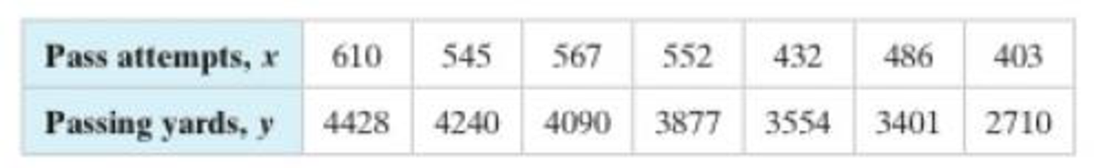
1. The numbers of pass attempts and passing yards for seven professional quarterbacks for a recent regular season (Sourer: National Football League)
a.
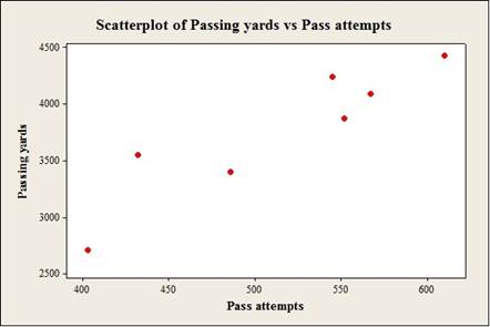
To construct: The scatterplot for the variables the numbers of pass attempts and passing yards.
Answer to Problem 9.1.1RE
Output using the MINITAB software is given below:
Explanation of Solution
Given info:
The data shows the numbers of pass attempts (x) and passing yards (y) values.
Calculation:
Software procedure:
Step by step procedure to obtain scatterplot using the MINITAB software:
- Choose Graph > Scatterplot.
- Choose Simple and then click OK.
- Under Y variables, enter a column of Passing yards.
- Under X variables, enter a column of Pass attempts.
- Click OK.
From the scatterplot, it is observed that as pass attempts increases, the passing yards also increases.
b.
To find: The value of the linear correlation coefficient r.
Answer to Problem 9.1.1RE
The linear correlation coefficient r is 0.917.
Explanation of Solution
Calculation:
Correlation coefficient r:
Software procedure:
Step-by-step procedure to obtain the ‘correlation coefficient’ using the MINITAB software:
- Select Stat > Basic Statistics > Correlation.
- In Variables, select Pass attempts and Passing yards from the box on the left.
- Click OK.
Output using the MINITAB software is given below:
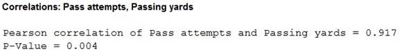
Thus, the Pearson correlation of the numbers of pass attempts and passing yards is 0.917 and P-value is 0.004.
c.
To describe: The type of linear association between the numbers of pass attempts and passing yards.
To interpret: The linear association between the numbers of pass attempts and passing yards.
Answer to Problem 9.1.1RE
There is a strong positive linear correlation between the numbers of pass attempts and passing yards.
As the numbers of pass attempts increase then the passing yards also increase.
Explanation of Solution
From, the scatterplot in part (a), it is observed that the horizontal axis represents the numbers of pass attempts and vertical axis represents the numbers of the passing yards. Also, it is observed that the numbers of pass attempts increase then the passing yards also increase. Also, the data points are scattered closely.
From part (b), it is observed that the linear correlation between the numbers of pass attempts and passing yards is 0.917.
Thus, there is a strong positive linear correlation between the numbers of pass attempts and passing yards
Want to see more full solutions like this?
Chapter 9 Solutions
Elementary Statistics: Picturing the World (7th Edition)


- I need help with this problem and an explanation of the solution for the image described below. (Statistics: Engineering Probabilities)arrow_forwardA survey of 250 young professionals found that two-thirds of them use their cell phones primarily for e-mail. Can you conclude statistically that the population proportion who use cell phones primarily for e-mail is less than 0.72? Use a 95% confidence interval. Question content area bottom Part 1 The 95% confidence interval is [ ], [ ] As 0.72 is ▼ above the upper limit within the limits below the lower limit of the confidence interval, we ▼ can cannot conclude that the population proportion is less than 0.72. (Use ascending order. Round to four decimal places as needed.)arrow_forwardI need help with this problem and an explanation of the solution for the image described below. (Statistics: Engineering Probabilities)arrow_forward
- I need help with this problem and an explanation of the solution for the image described below. (Statistics: Engineering Probabilities)arrow_forwardI need help with this problem and an explanation of the solution for the image described below. (Statistics: Engineering Probabilities)arrow_forwardQuestions An insurance company's cumulative incurred claims for the last 5 accident years are given in the following table: Development Year Accident Year 0 2018 1 2 3 4 245 267 274 289 292 2019 255 276 288 294 2020 265 283 292 2021 263 278 2022 271 It can be assumed that claims are fully run off after 4 years. The premiums received for each year are: Accident Year Premium 2018 306 2019 312 2020 318 2021 326 2022 330 You do not need to make any allowance for inflation. 1. (a) Calculate the reserve at the end of 2022 using the basic chain ladder method. (b) Calculate the reserve at the end of 2022 using the Bornhuetter-Ferguson method. 2. Comment on the differences in the reserves produced by the methods in Part 1.arrow_forward
- Questions An insurance company's cumulative incurred claims for the last 5 accident years are given in the following table: Development Year Accident Year 0 2018 1 2 3 4 245 267 274 289 292 2019 255 276 288 294 2020 265 283 292 2021 263 278 2022 271 It can be assumed that claims are fully run off after 4 years. The premiums received for each year are: Accident Year Premium 2018 306 2019 312 2020 318 2021 326 2022 330 You do not need to make any allowance for inflation. 1. (a) Calculate the reserve at the end of 2022 using the basic chain ladder method. (b) Calculate the reserve at the end of 2022 using the Bornhuetter-Ferguson method. 2. Comment on the differences in the reserves produced by the methods in Part 1.arrow_forwardFrom a sample of 26 graduate students, the mean number of months of work experience prior to entering an MBA program was 34.67. The national standard deviation is known to be18 months. What is a 90% confidence interval for the population mean? Question content area bottom Part 1 A 9090% confidence interval for the population mean is left bracket nothing comma nothing right bracketenter your response here,enter your response here. (Use ascending order. Round to two decimal places as needed.)arrow_forwardA test consists of 10 questions made of 5 answers with only one correct answer. To pass the test, a student must answer at least 8 questions correctly. (a) If a student guesses on each question, what is the probability that the student passes the test? (b) Find the mean and standard deviation of the number of correct answers. (c) Is it unusual for a student to pass the test by guessing? Explain.arrow_forward
- In a group of 40 people, 35% have never been abroad. Two people are selected at random without replacement and are asked about their past travel experience. a. Is this a binomial experiment? Why or why not? What is the probability that in a random sample of 2, no one has been abroad? b. What is the probability that in a random sample of 2, at least one has been abroad?arrow_forwardQuestions An insurance company's cumulative incurred claims for the last 5 accident years are given in the following table: Development Year Accident Year 0 2018 1 2 3 4 245 267 274 289 292 2019 255 276 288 294 2020 265 283 292 2021 263 278 2022 271 It can be assumed that claims are fully run off after 4 years. The premiums received for each year are: Accident Year Premium 2018 306 2019 312 2020 318 2021 326 2022 330 You do not need to make any allowance for inflation. 1. (a) Calculate the reserve at the end of 2022 using the basic chain ladder method. (b) Calculate the reserve at the end of 2022 using the Bornhuetter-Ferguson method. 2. Comment on the differences in the reserves produced by the methods in Part 1.arrow_forwardTo help consumers in purchasing a laptop computer, Consumer Reports calculates an overall test score for each computer tested based upon rating factors such as ergonomics, portability, performance, display, and battery life. Higher overall scores indicate better test results. The following data show the average retail price and the overall score for ten 13-inch models (Consumer Reports website, October 25, 2012). Brand & Model Price ($) Overall Score Samsung Ultrabook NP900X3C-A01US 1250 83 Apple MacBook Air MC965LL/A 1300 83 Apple MacBook Air MD231LL/A 1200 82 HP ENVY 13-2050nr Spectre XT 950 79 Sony VAIO SVS13112FXB 800 77 Acer Aspire S5-391-9880 Ultrabook 1200 74 Apple MacBook Pro MD101LL/A 1200 74 Apple MacBook Pro MD313LL/A 1000 73 Dell Inspiron I13Z-6591SLV 700 67 Samsung NP535U3C-A01US 600 63 a. Select a scatter diagram with price as the independent variable. b. What does the scatter diagram developed in part (a) indicate about the relationship…arrow_forward
 Glencoe Algebra 1, Student Edition, 9780079039897...AlgebraISBN:9780079039897Author:CarterPublisher:McGraw Hill
 Holt Mcdougal Larson Pre-algebra: Student Edition...AlgebraISBN:9780547587776Author:HOLT MCDOUGALPublisher:HOLT MCDOUGAL
 Big Ideas Math A Bridge To Success Algebra 1: Stu...AlgebraISBN:9781680331141Author:HOUGHTON MIFFLIN HARCOURTPublisher:Houghton Mifflin Harcourt