Concept explainers
Videos
(a)
Construct a
(a)
Answer to Problem 6CRP
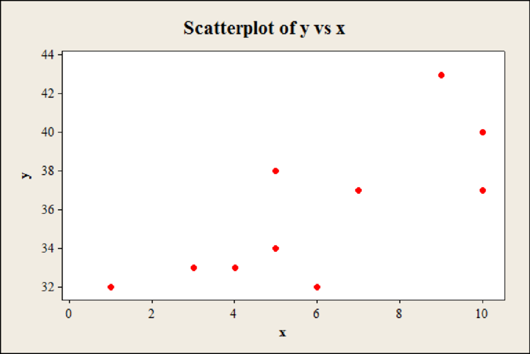
The scatter diagram for data is,
Explanation of Solution
Calculation:
The variable x denotes the number of job changes and y denotes the annual salary for people living in the Nashville area.
Step by step procedure to obtain scatter plot using MINITAB software is given below:
- Choose Graph > Scatterplot.
- Choose Simple. Click OK.
- In Y variables, enter the column of x.
- In X variables, enter the column of y.
- Click OK.
(b)
Find the value of
Find the value of
Find the value of b.
Find the equation of the least-squares line.
Construct the line on the scatter diagram.
(b)
Answer to Problem 6CRP
The value of
The value of
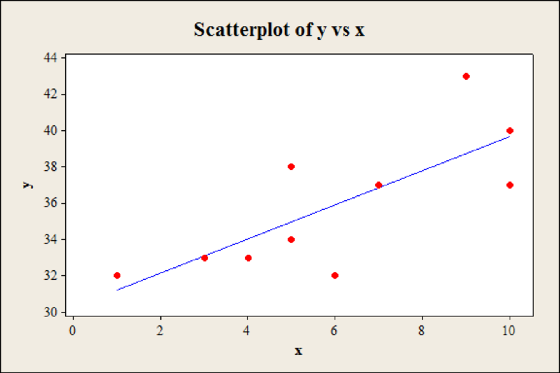
The value of b is 0.939.
The equation of the least-squares line is
The scatter plot the regression line is,
Explanation of Solution
Calculation:
The values are
The value of
Hence, the value of
The value of
Hence, the value of
The value of b is,
Hence, the value of b is 0.939024.
The value of a is,
The value of a is 30.266.
The equation of the least-squares line is,
Hence, the equation of the least-squares line is
Step by step procedure to obtain scatter plot using MINITAB software is given below:
- Choose Graph > Scatterplot.
- Choose With regression. Click OK.
- In Y variables, enter the column of x.
- In X variables, enter the column of y.
- Click OK.
(c)
Find the sample
Find the value of the coefficient of determination
Mention percentage of the variation in y is explained by the least-squares model.
(c)
Answer to Problem 6CRP
The sample
The value of the coefficient of determination
The percentage of the variation in y is explained by the least-squares model is 69.7%.
Explanation of Solution
Calculation:
Coefficient of determination
The coefficient of determination
Step by step procedure to obtain correlation using MINITAB software is given below:
- Choose Stat > Basic Statistics > Correlation.
- In Variable, enter the column as x, y.
- Click OK.
Output using MINITAB software is given below:
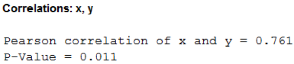
From MINITAB output, the correlation is 0.761.
Hence, the correlation coefficient r is 0.761.
The value of
Hence, the value of the coefficient of determination
About 57.9% of the variation in y (annual salary for people living in the Nashville area) is explained by x (number of job changes). Since the value of
Hence, the percentage of the variation in y that can be explained by variation in x is 57.9%.
(d)
Check whether the claim that the population correlation coefficient is positive or not.
(d)
Answer to Problem 6CRP
The population correlation coefficient is positive.
Explanation of Solution
Calculation:
Null hypothesis:
Alternative hypothesis:
Test statistic:
The test statistic formula for test correlation r is,
Where r is the sample correlation coefficient, n is the
Substitute r as 0.761, and n as 10 in the test statistic formula.
The test statistic value is 3.318.
The degrees of freedom is,
Step by step procedure to obtain P-value using MINITAB software is given below:
- Choose Graph > Probability Distribution Plot choose View Probability > OK.
- From Distribution, choose ‘t’ distribution.
- Enter the Degrees of freedom as 8.
- Click the Shaded Area tab.
- Choose X Value and Right Tail, for the region of the curve to shade.
- Enter the X value as 3.318.
- Click OK.
Output using MINITAB software is given below:
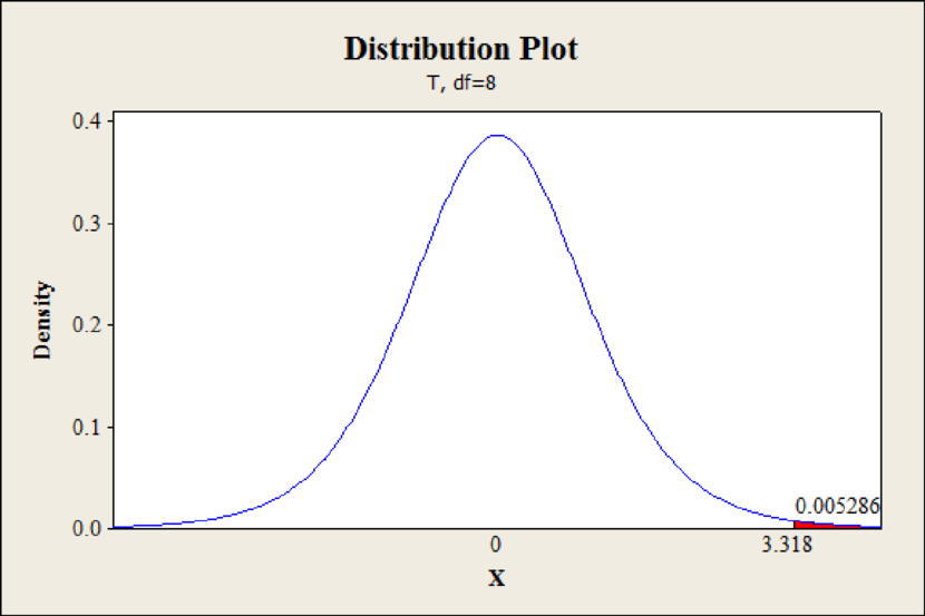
From Minitab output, the P-value is 0.0053.
Rejection rule:
- If the P-value is less than or equal to
Conclusion:
The P-value is 0.0053 and the level of significance is 0.05.
The P-value is less than the level of significance.
That is,
By the rejection rule, the null hypothesis is rejected.
Hence, the population correlation coefficient is positive between the number of job changes and annual salary for people living in the Nashville area.
(e)
Find the least-squares line predicts for y, the annual salary when
(e)
Answer to Problem 6CRP
The least-squares line predicts for y, the annual salary when
Explanation of Solution
Calculation:
From part (b), the equation of the least-squares line is
Substitute
Hence, the least-squares line predicts for y, the annual salary when
(f)
Verify the values of
(f)
Explanation of Solution
Calculation:
The value of
Hence, the value of
(g)
Find the 90% confidence interval for the annual salary of an individual with
(g)
Answer to Problem 6CRP
The 90% confidence interval for the annual salary of an individual with
Explanation of Solution
Calculation:
Step by step procedure to obtain confidence interval using MINITAB software is given below:
- Choose Stat > Regression > Regression.
- In Response, enter the column containing the response as y.
- In Predictors, enter the columns containing the predictor as x.
- Choose Options.
- In Prediction intervals for new observations, enter the value as 2.
- In Confidence level, enter value as 90.
- Click OK.
Output using MINITAB software is given below:
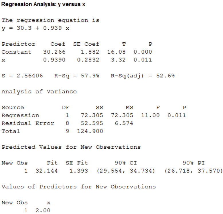
From Minitab output, the confidence interval is
Hence, the 90% confidence interval for the annual salary of an individual with
(h)
Check whether the claim that the slope
(h)
Answer to Problem 6CRP
The slope
Explanation of Solution
Calculation:
Null hypothesis:
Alternative hypothesis:
Test statistic:
From part (g) MINITAB output, the test statistic value is 3.32.
The degrees of freedom is,
Step by step procedure to obtain P-value using MINITAB software is given below:
- Choose Graph > Probability Distribution Plot choose View Probability > OK.
- From Distribution, choose ‘t’ distribution.
- Enter the Degrees of freedom as 8.
- Click the Shaded Area tab.
- Choose X Value and Right Tail, for the region of the curve to shade.
- Enter the X value as 3.32.
- Click OK.
Output using MINITAB software is given below:
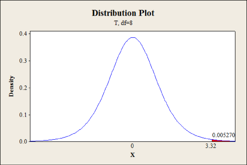
From Minitab output, the P-value is 0.0053.
Conclusion:
The P-value is 0.0053 and the level of significance is 0.05.
The P-value is less than the level of significance.
That is,
By the rejection rule, the null hypothesis is rejected.
Hence, the slope
(i)
Find a 90% confidence interval for
Interpret the confidence interval.
(i)
Answer to Problem 6CRP
The 90% confidence interval for
Explanation of Solution
Calculation:
Confidence interval for slope:
The confidence interval formula for slope
Where
Critical value:
Use the Appendix II: Tables, Table 6: Critical Values for Student’s t Distribution:
- In d.f. column locate the value 8.
- In the row of two-tail area locate the level of significance
- The intersecting value of row and columns is 1.860.
The critical value is
The margin of error is,
The 90% confidence interval for
Hence, the 90% confidence interval for
The annual salary for people living in the Nashville area increases by an amount that ranges between 0.413 and 1.465, if job changes increases by one unit.
Want to see more full solutions like this?
Chapter 9 Solutions
Understandable Statistics: Concepts and Methods


- ons 12. A sociologist hypothesizes that the crime rate is higher in areas with higher poverty rate and lower median income. She col- lects data on the crime rate (crimes per 100,000 residents), the poverty rate (in %), and the median income (in $1,000s) from 41 New England cities. A portion of the regression results is shown in the following table. Standard Coefficients error t stat p-value Intercept -301.62 549.71 -0.55 0.5864 Poverty 53.16 14.22 3.74 0.0006 Income 4.95 8.26 0.60 0.5526 a. b. Are the signs as expected on the slope coefficients? Predict the crime rate in an area with a poverty rate of 20% and a median income of $50,000. 3. Using data from 50 workarrow_forward2. The owner of several used-car dealerships believes that the selling price of a used car can best be predicted using the car's age. He uses data on the recent selling price (in $) and age of 20 used sedans to estimate Price = Po + B₁Age + ε. A portion of the regression results is shown in the accompanying table. Standard Coefficients Intercept 21187.94 Error 733.42 t Stat p-value 28.89 1.56E-16 Age -1208.25 128.95 -9.37 2.41E-08 a. What is the estimate for B₁? Interpret this value. b. What is the sample regression equation? C. Predict the selling price of a 5-year-old sedan.arrow_forwardian income of $50,000. erty rate of 13. Using data from 50 workers, a researcher estimates Wage = Bo+B,Education + B₂Experience + B3Age+e, where Wage is the hourly wage rate and Education, Experience, and Age are the years of higher education, the years of experience, and the age of the worker, respectively. A portion of the regression results is shown in the following table. ni ogolloo bash 1 Standard Coefficients error t stat p-value Intercept 7.87 4.09 1.93 0.0603 Education 1.44 0.34 4.24 0.0001 Experience 0.45 0.14 3.16 0.0028 Age -0.01 0.08 -0.14 0.8920 a. Interpret the estimated coefficients for Education and Experience. b. Predict the hourly wage rate for a 30-year-old worker with four years of higher education and three years of experience.arrow_forward
- 1. If a firm spends more on advertising, is it likely to increase sales? Data on annual sales (in $100,000s) and advertising expenditures (in $10,000s) were collected for 20 firms in order to estimate the model Sales = Po + B₁Advertising + ε. A portion of the regression results is shown in the accompanying table. Intercept Advertising Standard Coefficients Error t Stat p-value -7.42 1.46 -5.09 7.66E-05 0.42 0.05 8.70 7.26E-08 a. Interpret the estimated slope coefficient. b. What is the sample regression equation? C. Predict the sales for a firm that spends $500,000 annually on advertising.arrow_forwardCan you help me solve problem 38 with steps im stuck.arrow_forwardHow do the samples hold up to the efficiency test? What percentages of the samples pass or fail the test? What would be the likelihood of having the following specific number of efficiency test failures in the next 300 processors tested? 1 failures, 5 failures, 10 failures and 20 failures.arrow_forward
- The battery temperatures are a major concern for us. Can you analyze and describe the sample data? What are the average and median temperatures? How much variability is there in the temperatures? Is there anything that stands out? Our engineers’ assumption is that the temperature data is normally distributed. If that is the case, what would be the likelihood that the Safety Zone temperature will exceed 5.15 degrees? What is the probability that the Safety Zone temperature will be less than 4.65 degrees? What is the actual percentage of samples that exceed 5.25 degrees or are less than 4.75 degrees? Is the manufacturing process producing units with stable Safety Zone temperatures? Can you check if there are any apparent changes in the temperature pattern? Are there any outliers? A closer look at the Z-scores should help you in this regard.arrow_forwardNeed help pleasearrow_forwardPlease conduct a step by step of these statistical tests on separate sheets of Microsoft Excel. If the calculations in Microsoft Excel are incorrect, the null and alternative hypotheses, as well as the conclusions drawn from them, will be meaningless and will not receive any points. 4. One-Way ANOVA: Analyze the customer satisfaction scores across four different product categories to determine if there is a significant difference in means. (Hints: The null can be about maintaining status-quo or no difference among groups) H0 = H1=arrow_forward
- Please conduct a step by step of these statistical tests on separate sheets of Microsoft Excel. If the calculations in Microsoft Excel are incorrect, the null and alternative hypotheses, as well as the conclusions drawn from them, will be meaningless and will not receive any points 2. Two-Sample T-Test: Compare the average sales revenue of two different regions to determine if there is a significant difference. (Hints: The null can be about maintaining status-quo or no difference among groups; if alternative hypothesis is non-directional use the two-tailed p-value from excel file to make a decision about rejecting or not rejecting null) H0 = H1=arrow_forwardPlease conduct a step by step of these statistical tests on separate sheets of Microsoft Excel. If the calculations in Microsoft Excel are incorrect, the null and alternative hypotheses, as well as the conclusions drawn from them, will be meaningless and will not receive any points 3. Paired T-Test: A company implemented a training program to improve employee performance. To evaluate the effectiveness of the program, the company recorded the test scores of 25 employees before and after the training. Determine if the training program is effective in terms of scores of participants before and after the training. (Hints: The null can be about maintaining status-quo or no difference among groups; if alternative hypothesis is non-directional, use the two-tailed p-value from excel file to make a decision about rejecting or not rejecting the null) H0 = H1= Conclusion:arrow_forwardPlease conduct a step by step of these statistical tests on separate sheets of Microsoft Excel. If the calculations in Microsoft Excel are incorrect, the null and alternative hypotheses, as well as the conclusions drawn from them, will be meaningless and will not receive any points. The data for the following questions is provided in Microsoft Excel file on 4 separate sheets. Please conduct these statistical tests on separate sheets of Microsoft Excel. If the calculations in Microsoft Excel are incorrect, the null and alternative hypotheses, as well as the conclusions drawn from them, will be meaningless and will not receive any points. 1. One Sample T-Test: Determine whether the average satisfaction rating of customers for a product is significantly different from a hypothetical mean of 75. (Hints: The null can be about maintaining status-quo or no difference; If your alternative hypothesis is non-directional (e.g., μ≠75), you should use the two-tailed p-value from excel file to…arrow_forward
 Functions and Change: A Modeling Approach to Coll...AlgebraISBN:9781337111348Author:Bruce Crauder, Benny Evans, Alan NoellPublisher:Cengage Learning
 Linear Algebra: A Modern IntroductionAlgebraISBN:9781285463247Author:David PoolePublisher:Cengage Learning