
Subpart (a):
Calculate different costs.
Subpart (a):
Explanation of Solution
Total cost (TC) can be obtained by using the following formula.
Total cost at production level 1 unit can be calculated by substituting the respective values in Equation (1).
Total cost is $105.
Average fixed cost (AFC) can be obtained by using the following formula.
Average fixed cost at production level 1 unit can be calculated by substituting the respective values in Equation (2).
Average fixed cost is $60.
Average variable cost at production level 1 unit can be calculated by substituting the respective values in Equation (3).
Average variable cost is $45.
Total average cost (AC) can be obtained by using the following formula.
Total average cost at production level 1 unit can be calculated by substituting the respective values in Equation (4).
Average variable cost is $105.
Marginal cost (MC) can be obtained by using the following formula.
Average variable cost at production level 1 unit can be calculated by substituting the respective values in Equation (5).
Marginal cost is $105.
Table-1 shows the total cost, average fixed cost, average variable cost,
Table -1
| Quantity | Fixed cost | Variable cost | TC | AFC | AVC | AC | MC |
| 0 | 60 | 0 | 60 | ||||
| 1 | 60 | 45 | 105 | 60 | 45.00 | 105.00 | 45 |
| 2 | 60 | 85 | 145 | 30 | 42.50 | 72.50 | 40 |
| 3 | 60 | 120 | 180 | 20 | 40.00 | 60.00 | 35 |
| 4 | 60 | 150 | 210 | 15 | 37.50 | 52.50 | 30 |
| 5 | 60 | 185 | 245 | 12 | 37.00 | 49.00 | 35 |
| 6 | 60 | 225 | 285 | 10 | 37.50 | 47.50 | 40 |
| 7 | 60 | 270 | 330 | 8.57 | 38.57 | 47.14 | 45 |
| 8 | 60 | 325 | 385 | 7.50 | 40.63 | 48.13 | 55 |
| 9 | 60 | 390 | 450 | 6.67 | 43.33 | 50.00 | 65 |
| 10 | 60 | 465 | 525 | 6 | 46.50 | 52.50 | 75 |
Figure -1 illustrates the shape of total fixed cost, total cost and total variable cost that influencing by the diminishing returns to scale.
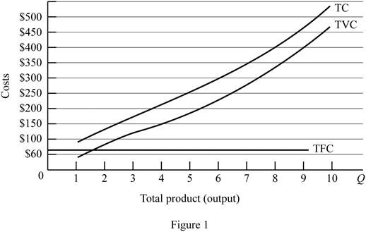
In figure -1, horizontal axis measures total output and vertical axis measures cost. The curve TC indicates total cost and the curve TVC indicates total variable cost. TFC curve indicates total fixed cost. Since total fixed cost is remain the same over the different level of production TFC curve parallel to the horizontal axis.
From the output range 1 unit to 4 units, total cost and total variable cost increasing at decreasing rate due to the increasing marginal returns. Thereafter, these two cost curves are increasing at increasing rate due to the diminishing marginal cost.
Concept introduction:
Fixed cost: Fixed costs refer to those costs that remain the same regardless of the level of production.
Variable cost: Variable cost refers to the costs that change due to the changes occurring in the level of production.
Subpart (b):
Calculate different costs.
Subpart (b):
Explanation of Solution
Figure -2 illustrates relationship between marginal cost, average variable cost, average fixed cost and average total cost curve.
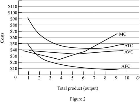
In figure -2, horizontal axis measures total output and vertical axis measures cost. The curve TC indicates total cost and the curve TVC indicates total variable cost. TFC curve indicates total fixed cost. Since total fixed cost is remain the same over the different level of production TFC curve parallel to the horizontal axis.
Since the fixed cost is spread over all the output, increasing the level of output leads to reduce the average fixed cost over the increasing production. Marginal cost curve average variable cost curve and average total cost curve are U shaped due to the operation of economies of scale and diseconomies of scale.
Average total cost curve is the vertical summation of average fixed cost and average variable cost. When the marginal cost curve is below to the average total cost curve, then the average total cost falls. When the marginal cost lies above the average total cost curve then the average total cost curve start rises. Thus, marginal cost curve intersects with the average total cost curve at the minimum point.
When the marginal cost curve is below to the average variable cost curve, then the average variable cost falls. When the marginal cost lies above the average variable cost curve then the average variable cost curve start rises. Thus, marginal cost curve intersects with the average variable cost curve at the minimum point.
Concept introduction:
Fixed cost: Fixed costs refer to those costs that remain the same regardless of the level of production.
Variable cost: Variable cost refers to the costs that change due to the changes occurring in the level of production.
Subpart (c):
Fixed cost and variable cost.
Subpart (c):
Explanation of Solution
The increasing fixed cost from $60 to $100 leads to shifts the fixed cost curve upward (By $40). This increasing fixed cost does not affect the marginal cost. Thus, marginal cost curve and average variable cost curve remains the same.
The decrease in variable cost by $10 leads to reduce the marginal cost $10 at first level of output and remains the same for other level of output. Average total cost and average variable cost decreases as a result of decrease in the variable cost. But, average fixed cost remains the same.
Concept introduction:
Fixed cost: Fixed costs refer to those costs that remain the same regardless of the level of production.
Variable cost: Variable cost refers to the costs that change due to the changes occurring in the level of production.
Want to see more full solutions like this?
Chapter 9 Solutions
Micro Economics / Macro Economics Spokane Falls Commnity College SFCC Econ 201/202

- Some people say that since inflation can be reduced in the long run without an increase in unemployment, we should reduce inflation to zero. Others believe that a steady rate of inflation at, say, 3 percent, should be our goal. What are the pros and cons of these two arguments? What, in your opinion, are good long-run goals for reducing inflation and unemployment?arrow_forwardExplain in words how investment multiplier and the interest sensitivity of aggregate demand affect the slope of the IS curve. Explain in words how and why the income and interest sensitivities of the demand for real balances affect the slope of the LM curve. According to the IS–LM model, what happens to the interest rate, income, consumption, and investment under the following circumstances?a. The central bank increases the money supply.b. The government increases government purchases.c. The government increases taxes.arrow_forwardSuppose that a person’s wealth is $50,000 and that her yearlyincome is $60,000. Also suppose that her money demand functionis given by Md = $Y10.35 - i2Derive the demand for bonds. Suppose the interest rate increases by 10 percentage points. What is the effect on her demand for bonds?b. What are the effects of an increase in income on her demand for money and her demand for bonds? Explain in wordsarrow_forward
- Imagine you are a world leader and you just viewed this presentation as part of the United Nations Sustainable Development Goal Meeting. Summarize your findings https://www.youtube.com/watch?v=v7WUpgPZzpIarrow_forwardPlease draw a standard Commercial Bank Balance Sheet and briefly explain each of the main components.arrow_forwardPlease draw the Federal Reserve System’s Balance Sheet and briefly explain each of the main components.arrow_forward
- 19. In a paragraph, no bullet, points please answer the question and follow the instructions. Give only the solution: Use the Feynman technique throughout. Assume that you’re explaining the answer to someone who doesn’t know the topic at all. How does the Federal Reserve currently get the federal funds rate where they want it to be?arrow_forward18. In a paragraph, no bullet, points please answer the question and follow the instructions. Give only the solution: Use the Feynman technique throughout. Assume that you’re explaining the answer to someone who doesn’t know the topic at all. Carefully compare and contrast fiscal policy and monetary policy.arrow_forward15. In a paragraph, no bullet, points please answer the question and follow the instructions. Give only the solution: Use the Feynman technique throughout. Assume that you’re explaining the answer to someone who doesn’t know the topic at all. What are the common arguments for and against high levels of federal debt?arrow_forward
- 17. In a paragraph, no bullet, points please answer the question and follow the instructions. Give only the solution: Use the Feynman technique throughout. Assume that you’re explaining the answer to someone who doesn’t know the topic at all. Explain the difference between present value and future value. Be sure to use and explain the mathematical formulas for both. How does one interpret these formulas?arrow_forward12. Give the solution: Use the Feynman technique throughout. Assume that you’re explaining the answer to someone who doesn’t know the topic at all. Show and carefully explain the Taylor rule and all of its components, used as a monetary policy guide.arrow_forward20. In a paragraph, no bullet, points please answer the question and follow the instructions. Give only the solution: Use the Feynman technique throughout. Assume that you’re explaining the answer to someone who doesn’t know the topic at all. What is meant by the Federal Reserve’s new term “ample reserves”? What may be hidden in this new formulation by the Fed?arrow_forward

 Economics (MindTap Course List)EconomicsISBN:9781337617383Author:Roger A. ArnoldPublisher:Cengage Learning


 Principles of Economics 2eEconomicsISBN:9781947172364Author:Steven A. Greenlaw; David ShapiroPublisher:OpenStax