
Subpart (a):
Calculate different costs.
Subpart (a):
Explanation of Solution
Total cost (TC) can be obtained by using the following formula.
Total cost at production level 1 unit can be calculated by substituting the respective values in Equation (1).
Total cost is $105.
Average fixed cost (AFC) can be obtained by using the following formula.
Average fixed cost at production level 1 unit can be calculated by substituting the respective values in Equation (2).
Average fixed cost is $60.
Average variable cost at production level 1 unit can be calculated by substituting the respective values in Equation (3).
Average variable cost is $45.
Total average cost (AC) can be obtained by using the following formula.
Total average cost at production level 1 unit can be calculated by substituting the respective values in Equation (4).
Average variable cost is $105.
Marginal cost (MC) can be obtained by using the following formula.
Average variable cost at production level 1 unit can be calculated by substituting the respective values in Equation (5).
Marginal cost is $105.
Table-1 shows the total cost, average fixed cost, average variable cost,
Table -1
| Quantity | Fixed cost | Variable cost | TC | AFC | AVC | AC | MC |
| 0 | 60 | 0 | 60 | ||||
| 1 | 60 | 45 | 105 | 60 | 45.00 | 105.00 | 45 |
| 2 | 60 | 85 | 145 | 30 | 42.50 | 72.50 | 40 |
| 3 | 60 | 120 | 180 | 20 | 40.00 | 60.00 | 35 |
| 4 | 60 | 150 | 210 | 15 | 37.50 | 52.50 | 30 |
| 5 | 60 | 185 | 245 | 12 | 37.00 | 49.00 | 35 |
| 6 | 60 | 225 | 285 | 10 | 37.50 | 47.50 | 40 |
| 7 | 60 | 270 | 330 | 8.57 | 38.57 | 47.14 | 45 |
| 8 | 60 | 325 | 385 | 7.50 | 40.63 | 48.13 | 55 |
| 9 | 60 | 390 | 450 | 6.67 | 43.33 | 50.00 | 65 |
| 10 | 60 | 465 | 525 | 6 | 46.50 | 52.50 | 75 |
Figure -1 illustrates the shape of total fixed cost, total cost and total variable cost that influencing by the diminishing returns to scale.
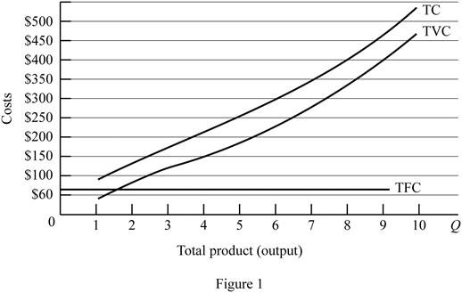
In figure -1, horizontal axis measures total output and vertical axis measures cost. The curve TC indicates total cost and the curve TVC indicates total variable cost. TFC curve indicates total fixed cost. Since total fixed cost is remain the same over the different level of production TFC curve parallel to the horizontal axis.
From the output range 1 unit to 4 units, total cost and total variable cost increasing at decreasing rate due to the increasing marginal returns. Thereafter, these two cost curves are increasing at increasing rate due to the diminishing marginal cost.
Concept introduction:
Fixed cost: Fixed costs refer to those costs that remain the same regardless of the level of production.
Variable cost: Variable cost refers to the costs that change due to the changes occurring in the level of production.
Subpart (b):
Calculate different costs.
Subpart (b):
Explanation of Solution
Figure -2 illustrates relationship between marginal cost, average variable cost, average fixed cost and average total cost curve.
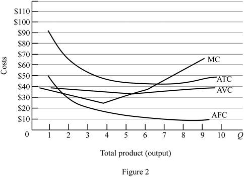
In figure -2, horizontal axis measures total output and vertical axis measures cost. The curve TC indicates total cost and the curve TVC indicates total variable cost. TFC curve indicates total fixed cost. Since total fixed cost is remain the same over the different level of production TFC curve parallel to the horizontal axis.
Since the fixed cost is spread over all the output, increasing the level of output leads to reduce the average fixed cost over the increasing production. Marginal cost curve average variable cost curve and average total cost curve are U shaped due to the operation of economies of scale and diseconomies of scale.
Average total cost curve is the vertical summation of average fixed cost and average variable cost. When the marginal cost curve is below to the average total cost curve, then the average total cost falls. When the marginal cost lies above the average total cost curve then the average total cost curve start rises. Thus, marginal cost curve intersects with the average total cost curve at the minimum point.
When the marginal cost curve is below to the average variable cost curve, then the average variable cost falls. When the marginal cost lies above the average variable cost curve then the average variable cost curve start rises. Thus, marginal cost curve intersects with the average variable cost curve at the minimum point.
Concept introduction:
Fixed cost: Fixed costs refer to those costs that remain the same regardless of the level of production.
Variable cost: Variable cost refers to the costs that change due to the changes occurring in the level of production.
Subpart (c):
Fixed cost and variable cost.
Subpart (c):
Explanation of Solution
The increasing fixed cost from $60 to $100 leads to shifts the fixed cost curve upward (By $40). This increasing fixed cost does not affect the marginal cost. Thus, marginal cost curve and average variable cost curve remains the same.
The decrease in variable cost by $10 leads to reduce the marginal cost $10 at first level of output and remains the same for other level of output. Average total cost and average variable cost decreases as a result of decrease in the variable cost. But, average fixed cost remains the same.
Concept introduction:
Fixed cost: Fixed costs refer to those costs that remain the same regardless of the level of production.
Variable cost: Variable cost refers to the costs that change due to the changes occurring in the level of production.
Want to see more full solutions like this?
Chapter 9 Solutions
Economics (Irwin Economics)

- Answerarrow_forwardM” method Given the following model, solve by the method of “M”. (see image)arrow_forwardAs indicated in the attached image, U.S. earnings for high- and low-skill workers as measured by educational attainment began diverging in the 1980s. The remaining questions in this problem set use the model for the labor market developed in class to walk through potential explanations for this trend. 1. Assume that there are just two types of workers, low- and high-skill. As a result, there are two labor markets: supply and demand for low-skill workers and supply and demand for high-skill workers. Using two carefully drawn labor-market figures, show that an increase in the demand for high skill workers can explain an increase in the relative wage of high-skill workers. 2. Using the same assumptions as in the previous question, use two carefully drawn labor-market figures to show that an increase in the supply of low-skill workers can explain an increase in the relative wage of high-skill workers.arrow_forward
- Published in 1980, the book Free to Choose discusses how economists Milton Friedman and Rose Friedman proposed a one-sided view of the benefits of a voucher system. However, there are other economists who disagree about the potential effects of a voucher system.arrow_forwardThe following diagram illustrates the demand and marginal revenue curves facing a monopoly in an industry with no economies or diseconomies of scale. In the short and long run, MC = ATC. a. Calculate the values of profit, consumer surplus, and deadweight loss, and illustrate these on the graph. b. Repeat the calculations in part a, but now assume the monopoly is able to practice perfect price discrimination.arrow_forwardThe projects under the 'Build, Build, Build' program: how these projects improve connectivity and ease of doing business in the Philippines?arrow_forward

 Economics (MindTap Course List)EconomicsISBN:9781337617383Author:Roger A. ArnoldPublisher:Cengage Learning


 Principles of Economics 2eEconomicsISBN:9781947172364Author:Steven A. Greenlaw; David ShapiroPublisher:OpenStax