
Sub- Part
A
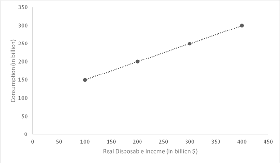
Based on the data, Graphical representation of consumption function, with consumption spending on vertical axis and disposable income on horizontal axis.
Sub- Part
A
Explanation of Solution
(a) − Following graph shows the consumption function in an economy.
Sub- Part
Introduction: Consumption function represents the functional relationship between total consumption and gross
B
Based on the data, to find:
Slope, if consumption function is a straight line
B
Explanation of Solution
In case of a straight line, slope of the line remains constant or same everywhere along the line. So, if the consumption function is a straight line then its slope will remain same everywhere along it. The difference between two level of income and consumption will be constant. The slope of consumption function can be calculates as follows −


Thus, the slope of given consumption function is 0.5.
Sub- Part
Introduction: Consumption function represents the functional relationship between total consumption and gross national income. Consumer spending depends on three factors: disposable income (Yd), autonomous consumption (a), i.e. when income is zero, and induced income (b), i.e. the percentage of extra income that is spent. The formula for the same is C = a + b*Yd.
C
Based on the data,
Find the Savings at each level of income and the slope when the saving function is a straight line.
C
Explanation of Solution
If the saving function is a straight line then its slope will remain constant. Difference between two level of income and saving will remain constant along the saving function. As saving function is a straight line, change in saving and income would be the same. Thus, the slope of saving function would be:


| Real Disposable Income (in billion $) | Consumption Expenditure (in billion $) | Savings (in billion $) |
| 100 | 150 | -50 |
| 200 | 200 | 0 |
| 300 | 250 | 50 |
| 400 | 300 | 100 |
Introduction: Consumption function represents the functional relationship between total consumption and gross national income. Consumer spending depends on three factors: disposable income (Yd), autonomous consumption (a), i.e. when income is zero, and induced income (b), i.e. the percentage of extra income that is spent. The formula for the same is C = a + b*Yd.
Want to see more full solutions like this?

- What is the primary, secondary, tertiary, and quaternary levels of mining in Canada For each level, describe what types of careers are the most common, and describe what stage your industry’s main resource is in during that stagearrow_forwardHow does the mining industry in canada contribute to the Canadian economy? Describe why your industry is so important to the Canadian economy What would happen if your industry disappeared, or suffered significant layoffs?arrow_forwardWhat is already being done to make mining in canada more sustainable? What efforts are being made in order to make mining more sustainable?arrow_forward
- What are the environmental challenges the canadian mining industry face? Discuss current challenges that mining faces with regard to the environmentarrow_forwardWhat sustainability efforts have been put forth in the mining industry in canada Are your industry’s resources renewable or non-renewable? How do you know? Describe your industry’s reclamation processarrow_forwardHow does oligopolies practice non-price competition in South Africa?arrow_forward
- What are the advantages and disadvantages of oligopolies on the consumers, businesses and the economy as a whole?arrow_forward1. After the reopening of borders with mainland China following the COVID-19 lockdown, residents living near the border now have the option to shop for food on either side. In Hong Kong, the cost of food is at its listed price, while across the border in mainland China, the price is only half that of Hong Kong's. A recent report indicates a decline in food sales in Hong Kong post-reopening. ** Diagrams need not be to scale; Focus on accurately representing the relevant concepts and relationships rather than the exact proportions. (a) Using a diagram, explain why Hong Kong's food sales might have dropped after the border reopening. Assume that consumers are indifferent between purchasing food in Hong Kong or mainland China, and therefore, their indifference curves have a slope of one like below. Additionally, consider that there are no transport costs and the daily food budget for consumers is identical whether they shop in Hong Kong or mainland China. I 3. 14 (b) In response to the…arrow_forward2. Health Food Company is a well-known global brand that specializes in healthy and organic food products. One of their main products is organic chicken, which they source from small farmers in the area. Health Food Company is the sole buyer of organic chicken in the market. (a) In the context of the organic chicken industry, what type of market structure is Health Food Company operating in? (b) Using a diagram, explain how the identified market structure affects the input pricing and output decisions of Health Food Company. Specifically, include the relevant curves and any key points such as the profit-maximizing price and quantity. () (c) How can encouraging small chicken farmers to form bargaining associations help improve their trade terms? Explain how this works by drawing on the graph in answer (b) to illustrate your answer.arrow_forward
- 2. Suppose that a farmer has two ways to produce his crop. He can use a low-polluting technology with the marginal cost curve MCL or a high polluting technology with the marginal cost curve MCH. If the farmer uses the high-polluting technology, for each unit of quantity produced, one unit of pollution is also produced. Pollution causes pollution damages that are valued at $E per unit. The good produced can be sold in the market for $P per unit. P 1 MCH 0 Q₁ MCL Q2 E a. b. C. If there are no restrictions on the firm's choices, which technology will the farmer use and what quantity will he produce? Explain, referring to the area identified in the figure Given your response in part a, is it socially efficient for there to be no restriction on production? Explain, referring to the area identified in the figure If the government restricts production to Q1, what technology would the farmer choose? Would a socially efficient outcome be achieved? Explain, referring to the area identified in…arrow_forwardI need help in seeing how these are the answers. If you could please write down your steps so I can see how it's done please.arrow_forwardSuppose that a random sample of 216 twenty-year-old men is selected from a population and that their heights and weights are recorded. A regression of weight on height yields Weight = (-107.3628) + 4.2552 x Height, R2 = 0.875, SER = 11.0160 (2.3220) (0.3348) where Weight is measured in pounds and Height is measured in inches. A man has a late growth spurt and grows 1.6200 inches over the course of a year. Construct a confidence interval of 90% for the person's weight gain. The 90% confidence interval for the person's weight gain is ( ☐ ☐) (in pounds). (Round your responses to two decimal places.)arrow_forward

 Essentials of Economics (MindTap Course List)EconomicsISBN:9781337091992Author:N. Gregory MankiwPublisher:Cengage Learning
 Brief Principles of Macroeconomics (MindTap Cours...EconomicsISBN:9781337091985Author:N. Gregory MankiwPublisher:Cengage Learning

