
To find:
A 99% confidence interval for the mean
Answer to Problem 14E
Solution:
A 99% confidence interval for the mean face amount of an individual life insurance policy is in the interval,
Explanation of Solution
Approach:
Given a sample with standard deviation
The true population parameters probability lies in this interval range which is known as the confidence level
At a certain level of confidence, the interval in which the maximum error can be observed is known as the confidence interval.
Estimating parameters of a large population or a population following
The
The degrees of freedom is the attribute used to obtain the appropriate curve for the
The value of
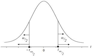
Hence this is a case of two-tailed t-distribution.
The maximum distance from point estimate that the confidence interval covers is margin of error and is given by:
Given the sample mean
Calculation:
The sample means is given by:
Substituting the values of life insurance policies in the formula above
| 150, 000 | 171758.62 | -21, 758.62 | 473437544.3 |
| 150, 000 | 171758.62 | -21, 758.62 | 473437544.3 |
| 150, 000 | 171758.62 | -21, 758.62 | 473437544.3 |
| 150, 000 | 171758.62 | -21, 758.62 | 473437544.3 |
| 150, 000 | 171758.62 | -21, 758.62 | 473437544.3 |
| 150, 000 | 171758.62 | -21, 758.62 | 473437544.3 |
| 151, 000 | 171758.62 | -20, 758.62 | 430920304.3 |
| 152, 000 | 171758.62 | -19, 758.62 | 390403064.3 |
| 152, 000 | 171758.62 | -19, 758.62 | 390403064.3 |
| 153, 000 | 171758.62 | -18, 758.62 | 351885824.3 |
| 153, 000 | 171758.62 | -18, 758.62 | 351885824.3 |
| 154, 000 | 171758.62 | -17, 758.62 | 315368584.3 |
| 155, 000 | 171758.62 | -16, 758.62 | 280851344.3 |
| 158, 000 | 171758.62 | -13, 758.62 | 189299624.3 |
| 158, 000 | 171758.62 | -12, 758.62 | 162782384.3 |
| 158, 000 | 171758.62 | -12, 758.62 | 162782384.3 |
| 160, 000 | 171758.62 | -11, 758.62 | 138265144.3 |
| 160, 000 | 171758.62 | -11, 758.62 | 138265144.3 |
| 160, 000 | 171758.62 | -11, 758.62 | 138265144.3 |
| 162, 000 | 171758.62 | -9, 758.62 | 95230664.3 |
| 163, 000 | 171758.62 | -8, 758.62 | 76713424.3 |
| 163, 000 | 171758.62 | -8, 758.62 | 76713424.3 |
| 163, 000 | 171758.62 | -8, 758.62 | 76713424.3 |
| 165, 000 | 171758.62 | -6, 758.62 | 45678944.3 |
| 165, 000 | 171758.62 | -6, 758.62 | 45678944.3 |
| 168, 000 | 171758.62 | -3, 758.62 | 14127224.3 |
| 168, 000 | 171758.62 | -3, 758.62 | 14127224.3 |
| 168, 000 | 171758.62 | -3, 758.62 | 14127224.3 |
| 171, 000 | 171758.62 | -758.62 | 575504.3044 |
| 171, 000 | 171758.62 | -758.62 | 575504.3044 |
| 172, 000 | 171758.62 | 241.38 | 58264.3044 |
| 172, 000 | 171758.62 | 241.38 | 58264.3044 |
| 172, 000 | 171758.62 | 241.38 | 58264.3044 |
| 173, 000 | 171758.62 | 1, 241.38 | 1541024.304 |
| 174, 000 | 171758.62 | 2, 241.38 | 5023784.304 |
| 175, 000 | 171758.62 | 3, 241.38 | 10506544.3 |
| 175, 000 | 171758.62 | 3, 241.38 | 10506544.3 |
| 175, 000 | 171758.62 | 3, 241.38 | 10506544.3 |
| 176, 000 | 171758.62 | 4, 241.38 | 17989304.3 |
| 182, 000 | 171758.62 | 10, 241.38 | 104885864.3 |
| 182, 000 | 171758.62 | 10, 241.38 | 104885864.3 |
| 183, 000 | 171758.62 | 11, 241.38 | 126368624.3 |
| 185, 000 | 171758.62 | 13, 241.38 | 175334144.3 |
| 185, 000 | 171758.62 | 13, 241.38 | 175334144.3 |
| 190, 000 | 171758.62 | 18, 241.38 | 332747944.3 |
| 190, 000 | 171758.62 | 18, 241.38 | 332747944.3 |
| 195, 000 | 171758.62 | 23, 241.38 | 540161744.3 |
| 195, 000 | 171758.62 | 23, 241.38 | 540161744.3 |
| 195, 000 | 171758.62 | 23, 241.38 | 540161744.3 |
| 196, 000 | 171758.62 | 24, 241.38 | 587644504.3 |
| 200, 000 | 171758.62 | 28, 241.38 | 797575544.3 |
| 200, 000 | 171758.62 | 28, 241.38 | 797575544.3 |
| 200, 000 | 171758.62 | 28, 241.38 | 797575544.3 |
| 200, 000 | 171758.62 | 28, 241.38 | 797575544.3 |
| 200, 000 | 171758.62 | 28, 241.38 | 797575544.3 |
| 202, 000 | 171758.62 | 30, 241.38 | 914541064.3 |
| 202, 000 | 171758.62 | 30, 241.38 | 914541064.3 |
| 163, 000 | 171758.62 | -8, 758.62 | 76713424.3 |
Form the above table we get,
Now the standard division is,
Level of confidence is 99%
Where
Critical t value at
Now substitute these values in margin of error.
Then, the margin of error is calculated as:
Then, interval is:
Conclusion:
A 95% confidence interval for the mean fastball pitching speed of all high school is in the interval
Want to see more full solutions like this?
Chapter 8 Solutions
BEGINNING STAT.-SOFTWARE+EBOOK ACCESS

- A survey of 250 young professionals found that two-thirds of them use their cell phones primarily for e-mail. Can you conclude statistically that the population proportion who use cell phones primarily for e-mail is less than 0.72? Use a 95% confidence interval. Question content area bottom Part 1 The 95% confidence interval is [ ], [ ] As 0.72 is ▼ above the upper limit within the limits below the lower limit of the confidence interval, we ▼ can cannot conclude that the population proportion is less than 0.72. (Use ascending order. Round to four decimal places as needed.)arrow_forwardI need help with this problem and an explanation of the solution for the image described below. (Statistics: Engineering Probabilities)arrow_forwardI need help with this problem and an explanation of the solution for the image described below. (Statistics: Engineering Probabilities)arrow_forward
- I need help with this problem and an explanation of the solution for the image described below. (Statistics: Engineering Probabilities)arrow_forwardQuestions An insurance company's cumulative incurred claims for the last 5 accident years are given in the following table: Development Year Accident Year 0 2018 1 2 3 4 245 267 274 289 292 2019 255 276 288 294 2020 265 283 292 2021 263 278 2022 271 It can be assumed that claims are fully run off after 4 years. The premiums received for each year are: Accident Year Premium 2018 306 2019 312 2020 318 2021 326 2022 330 You do not need to make any allowance for inflation. 1. (a) Calculate the reserve at the end of 2022 using the basic chain ladder method. (b) Calculate the reserve at the end of 2022 using the Bornhuetter-Ferguson method. 2. Comment on the differences in the reserves produced by the methods in Part 1.arrow_forwardQuestions An insurance company's cumulative incurred claims for the last 5 accident years are given in the following table: Development Year Accident Year 0 2018 1 2 3 4 245 267 274 289 292 2019 255 276 288 294 2020 265 283 292 2021 263 278 2022 271 It can be assumed that claims are fully run off after 4 years. The premiums received for each year are: Accident Year Premium 2018 306 2019 312 2020 318 2021 326 2022 330 You do not need to make any allowance for inflation. 1. (a) Calculate the reserve at the end of 2022 using the basic chain ladder method. (b) Calculate the reserve at the end of 2022 using the Bornhuetter-Ferguson method. 2. Comment on the differences in the reserves produced by the methods in Part 1.arrow_forward
- From a sample of 26 graduate students, the mean number of months of work experience prior to entering an MBA program was 34.67. The national standard deviation is known to be18 months. What is a 90% confidence interval for the population mean? Question content area bottom Part 1 A 9090% confidence interval for the population mean is left bracket nothing comma nothing right bracketenter your response here,enter your response here. (Use ascending order. Round to two decimal places as needed.)arrow_forwardA test consists of 10 questions made of 5 answers with only one correct answer. To pass the test, a student must answer at least 8 questions correctly. (a) If a student guesses on each question, what is the probability that the student passes the test? (b) Find the mean and standard deviation of the number of correct answers. (c) Is it unusual for a student to pass the test by guessing? Explain.arrow_forwardIn a group of 40 people, 35% have never been abroad. Two people are selected at random without replacement and are asked about their past travel experience. a. Is this a binomial experiment? Why or why not? What is the probability that in a random sample of 2, no one has been abroad? b. What is the probability that in a random sample of 2, at least one has been abroad?arrow_forward
- Questions An insurance company's cumulative incurred claims for the last 5 accident years are given in the following table: Development Year Accident Year 0 2018 1 2 3 4 245 267 274 289 292 2019 255 276 288 294 2020 265 283 292 2021 263 278 2022 271 It can be assumed that claims are fully run off after 4 years. The premiums received for each year are: Accident Year Premium 2018 306 2019 312 2020 318 2021 326 2022 330 You do not need to make any allowance for inflation. 1. (a) Calculate the reserve at the end of 2022 using the basic chain ladder method. (b) Calculate the reserve at the end of 2022 using the Bornhuetter-Ferguson method. 2. Comment on the differences in the reserves produced by the methods in Part 1.arrow_forwardTo help consumers in purchasing a laptop computer, Consumer Reports calculates an overall test score for each computer tested based upon rating factors such as ergonomics, portability, performance, display, and battery life. Higher overall scores indicate better test results. The following data show the average retail price and the overall score for ten 13-inch models (Consumer Reports website, October 25, 2012). Brand & Model Price ($) Overall Score Samsung Ultrabook NP900X3C-A01US 1250 83 Apple MacBook Air MC965LL/A 1300 83 Apple MacBook Air MD231LL/A 1200 82 HP ENVY 13-2050nr Spectre XT 950 79 Sony VAIO SVS13112FXB 800 77 Acer Aspire S5-391-9880 Ultrabook 1200 74 Apple MacBook Pro MD101LL/A 1200 74 Apple MacBook Pro MD313LL/A 1000 73 Dell Inspiron I13Z-6591SLV 700 67 Samsung NP535U3C-A01US 600 63 a. Select a scatter diagram with price as the independent variable. b. What does the scatter diagram developed in part (a) indicate about the relationship…arrow_forwardTo the Internal Revenue Service, the reasonableness of total itemized deductions depends on the taxpayer’s adjusted gross income. Large deductions, which include charity and medical deductions, are more reasonable for taxpayers with large adjusted gross incomes. If a taxpayer claims larger than average itemized deductions for a given level of income, the chances of an IRS audit are increased. Data (in thousands of dollars) on adjusted gross income and the average or reasonable amount of itemized deductions follow. Adjusted Gross Income ($1000s) Reasonable Amount ofItemized Deductions ($1000s) 22 9.6 27 9.6 32 10.1 48 11.1 65 13.5 85 17.7 120 25.5 Compute b1 and b0 (to 4 decimals).b1 b0 Complete the estimated regression equation (to 2 decimals). = + x Predict a reasonable level of total itemized deductions for a taxpayer with an adjusted gross income of $52.5 thousand (to 2 decimals). thousand dollarsWhat is the value, in dollars, of…arrow_forward
 MATLAB: An Introduction with ApplicationsStatisticsISBN:9781119256830Author:Amos GilatPublisher:John Wiley & Sons Inc
 Probability and Statistics for Engineering and th...StatisticsISBN:9781305251809Author:Jay L. DevorePublisher:Cengage Learning
 Statistics for The Behavioral Sciences (MindTap C...StatisticsISBN:9781305504912Author:Frederick J Gravetter, Larry B. WallnauPublisher:Cengage Learning
 Elementary Statistics: Picturing the World (7th E...StatisticsISBN:9780134683416Author:Ron Larson, Betsy FarberPublisher:PEARSON
 The Basic Practice of StatisticsStatisticsISBN:9781319042578Author:David S. Moore, William I. Notz, Michael A. FlignerPublisher:W. H. Freeman
 Introduction to the Practice of StatisticsStatisticsISBN:9781319013387Author:David S. Moore, George P. McCabe, Bruce A. CraigPublisher:W. H. Freeman