Pearson eText for Elementary Statistics: Picturing the World -- Instant Access (Pearson+)
7th Edition
ISBN: 9780137504329
Author: Ron Larson, Betsy Farber
Publisher: PEARSON+
expand_more
expand_more
format_list_bulleted
Videos
Textbook Question
Chapter 8.1, Problem 9E
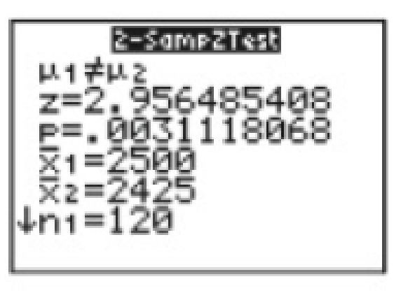
In Exercises 9 and 10, use the TI-H4 Plus display to make a decision to reject or fail to reject the null hypothesis at the level of significance. Make your decision using the standardized test statistic and using the P-value. Assume the
9. α = 0.05
Expert Solution & Answer

Trending nowThis is a popular solution!

Students have asked these similar questions
(c) Because logistic regression predicts probabilities of outcomes, observations used to build a logistic regression model need not be independent.
A. false: all observations must be independent
B. true
C. false: only observations with the same outcome need to be independent
I ANSWERED: A. false: all observations must be independent.
(This was marked wrong but I have no idea why. Isn't this a basic assumption of logistic regression)
Business discuss
Spam filters are built on principles similar to those used in logistic regression. We fit a probability that each message is spam or not spam. We have several variables for each email. Here are a few: to_multiple=1 if there are multiple recipients, winner=1 if the word 'winner' appears in the subject line, format=1 if the email is poorly formatted, re_subj=1 if "re" appears in the subject line. A logistic model was fit to a dataset with the following output:
Estimate
SE
Z
Pr(>|Z|)
(Intercept)
-0.8161
0.086
-9.4895
0
to_multiple
-2.5651
0.3052
-8.4047
0
winner
1.5801
0.3156
5.0067
0
format
-0.1528
0.1136
-1.3451
0.1786
re_subj
-2.8401
0.363
-7.824
0
(a) Write down the model using the coefficients from the model fit.log_odds(spam) = -0.8161 + -2.5651 + to_multiple + 1.5801 winner + -0.1528 format + -2.8401 re_subj(b) Suppose we have an observation where to_multiple=0, winner=1, format=0, and re_subj=0. What is the predicted probability that this message is spam?…
Chapter 8 Solutions
Pearson eText for Elementary Statistics: Picturing the World -- Instant Access (Pearson+)
Ch. 8.1 - Classify each pair of samples as independent or...Ch. 8.1 - A survey indicates that the mean annual wages for...Ch. 8.1 - A travel agency claims that the average daily cost...Ch. 8.1 - What is the difference between two samples that...Ch. 8.1 - Explain how to perform a two-sample z-test for the...Ch. 8.1 - Describe another way you can perform a hypothesis...Ch. 8.1 - What conditions are necessary in order to use the...Ch. 8.1 - Prob. 5ECh. 8.1 - Prob. 6ECh. 8.1 - Independent and Dependent Samples In Exercises 58,...
Ch. 8.1 - Prob. 8ECh. 8.1 - In Exercises 9 and 10, use the TI-H4 Plus display...Ch. 8.1 - Prob. 10ECh. 8.1 - Prob. 11ECh. 8.1 - In Exercises 1114, test the claim about the...Ch. 8.1 - In Exercises 1114, test the claim about the...Ch. 8.1 - Prob. 14ECh. 8.1 - Testing the Difference Between Two Means In...Ch. 8.1 - Testing the Difference Between Two Means In...Ch. 8.1 - Prob. 17ECh. 8.1 - Prob. 18ECh. 8.1 - Prob. 19ECh. 8.1 - Testing the Difference Between Two Means In...Ch. 8.1 - Testing the Difference Between Two Means In...Ch. 8.1 - Prob. 22ECh. 8.1 - Prob. 23ECh. 8.1 - Prob. 24ECh. 8.1 - Prob. 25ECh. 8.1 - Getting at the Concept Explain why the null...Ch. 8.1 - Testing a Difference Other Than Zero Sometimes a...Ch. 8.1 - Testing a Difference Other Than Zero Sometimes a...Ch. 8.1 - Prob. 29ECh. 8.1 - Architect Salaries Construct a 99% confidence...Ch. 8.2 - The annual earnings of 25 people with a high...Ch. 8.2 - A manufacturer claims that the mean driving cost...Ch. 8.2 - What conditions are necessary in order to use the...Ch. 8.2 - Explain how to perform a two-sample t-test for the...Ch. 8.2 - Prob. 3ECh. 8.2 - Prob. 4ECh. 8.2 - Prob. 5ECh. 8.2 - Prob. 6ECh. 8.2 - In Exercises 38, use Table 5 in Appendix B to find...Ch. 8.2 - Prob. 8ECh. 8.2 - In Exercises 912, test the claim about the...Ch. 8.2 - Prob. 10ECh. 8.2 - Prob. 11ECh. 8.2 - In Exercises 912, test the claim about the...Ch. 8.2 - Testing the Difference Between Two Means in...Ch. 8.2 - Testing the Difference Between Two Means in...Ch. 8.2 - Testing the Difference Between Two Means in...Ch. 8.2 - Testing the Difference Between Two Means in...Ch. 8.2 - Prob. 17ECh. 8.2 - Prob. 18ECh. 8.2 - Prob. 19ECh. 8.2 - Testing the Difference Between Two Means in...Ch. 8.2 - Testing the Difference Between Two Means in...Ch. 8.2 - Testing the Difference Between Two Means in...Ch. 8.2 - Constructing Confidence Intervals for 1 2 When...Ch. 8.2 - Constructing Confidence Intervals for 1 2 When...Ch. 8.2 - Constructing Confidence Intervals for 1 2 When...Ch. 8.2 - Prob. 26ECh. 8.2 - How Protein Affects Weight Gain in Overeaters In a...Ch. 8.2 - Prob. 2CSCh. 8.2 - How Protein Affects Weight Gain in Overeaters In a...Ch. 8.2 - Prob. 4CSCh. 8.2 - Prob. 5CSCh. 8.3 - A shoe manufacturer claims that athletes can...Ch. 8.3 - Prob. 2TYCh. 8.3 - Prob. 1ECh. 8.3 - Prob. 2ECh. 8.3 - Prob. 3ECh. 8.3 - Prob. 4ECh. 8.3 - Prob. 5ECh. 8.3 - Prob. 6ECh. 8.3 - Prob. 7ECh. 8.3 - Prob. 8ECh. 8.3 - Prob. 9ECh. 8.3 - Testing the Difference Between Two Means In...Ch. 8.3 - Prob. 11ECh. 8.3 - Prob. 12ECh. 8.3 - Prob. 13ECh. 8.3 - Testing the Difference Between Two Means In...Ch. 8.3 - Prob. 15ECh. 8.3 - Prob. 16ECh. 8.3 - Testing the Difference Between Two Means In...Ch. 8.3 - Testing the Difference Between Two Means In...Ch. 8.3 - Testing the Difference Between Two Means In...Ch. 8.3 - Prob. 20ECh. 8.3 - Prob. 21ECh. 8.3 - Prob. 22ECh. 8.3 - Prob. 23ECh. 8.3 - Prob. 24ECh. 8.4 - Consider the results of the study discussed on...Ch. 8.4 - Prob. 2TYCh. 8.4 - What conditions are necessary in order to use the...Ch. 8.4 - Explain how to perform a two-sample z-test for the...Ch. 8.4 - In Exercises 36, determine whether a normal...Ch. 8.4 - Prob. 4ECh. 8.4 - Prob. 5ECh. 8.4 - In Exercises 36, determine whether a normal...Ch. 8.4 - Prob. 7ECh. 8.4 - Testing the Difference Between Two Proportions In...Ch. 8.4 - Prob. 9ECh. 8.4 - Prob. 10ECh. 8.4 - Prob. 11ECh. 8.4 - Testing the Difference Between Two Proportions In...Ch. 8.4 - Prob. 13ECh. 8.4 - Prob. 14ECh. 8.4 - Intermarriages In Exercises 1318, use the figure,...Ch. 8.4 - Prob. 16ECh. 8.4 - Prob. 17ECh. 8.4 - Intermarriages In Exercises 1318, use the figure,...Ch. 8.4 - Prob. 19ECh. 8.4 - Prob. 20ECh. 8.4 - Prob. 21ECh. 8.4 - U.S. Workforce In Exercises 1922, use the figure...Ch. 8.4 - Prob. 23ECh. 8.4 - Prob. 24ECh. 8.4 - Prob. 25ECh. 8.4 - Prob. 26ECh. 8 - Uses Hypothesis Testing with Two Samples...Ch. 8 - Medical research often involves blind and...Ch. 8 - Prob. 8.1.1RECh. 8 - Prob. 8.1.2RECh. 8 - Sample 1: The fuel efficiencies of 20 sports...Ch. 8 - Prob. 8.1.4RECh. 8 - Prob. 8.1.5RECh. 8 - In Exercises 58, test the claim about the...Ch. 8 - Prob. 8.1.7RECh. 8 - In Exercises 58, test the claim about the...Ch. 8 - In Exercises 9 and 10, (a) identify the claim and...Ch. 8 - Prob. 8.1.10RECh. 8 - Prob. 8.2.11RECh. 8 - Prob. 8.2.12RECh. 8 - Prob. 8.2.13RECh. 8 - Prob. 8.2.14RECh. 8 - Prob. 8.2.15RECh. 8 - Prob. 8.2.16RECh. 8 - Prob. 8.2.17RECh. 8 - Prob. 8.2.18RECh. 8 - Prob. 8.3.19RECh. 8 - In Exercises 1922, test the claim about the mean...Ch. 8 - Prob. 8.3.21RECh. 8 - Prob. 8.3.22RECh. 8 - Prob. 8.3.23RECh. 8 - In Exercises 23 and 24, (a) identify the claim and...Ch. 8 - Prob. 8.4.25RECh. 8 - Prob. 8.4.26RECh. 8 - Prob. 8.4.27RECh. 8 - Prob. 8.4.28RECh. 8 - Prob. 8.4.29RECh. 8 - Prob. 8.4.30RECh. 8 - Prob. 1CQCh. 8 - Prob. 2CQCh. 8 - Prob. 3CQCh. 8 - Prob. 4CQCh. 8 - Take this test as you would take a test in class....Ch. 8 - Prob. 2CTCh. 8 - A physical therapist suggests that soft tissue...Ch. 8 - Take this test as you would take a test in class....Ch. 8 - The U.S. Department of Health Human Services...Ch. 8 - Prob. 2RSRDCh. 8 - Prob. 3RSRDCh. 8 - Prob. 4RSRDCh. 8 - Prob. 1TCh. 8 - Prob. 2TCh. 8 - Prob. 3TCh. 8 - Prob. 4TCh. 8 - Prob. 5TCh. 8 - Prob. 1CRCh. 8 - Prob. 2CRCh. 8 - Prob. 3CRCh. 8 - Prob. 4CRCh. 8 - In Exercises 36, construct the indicated...Ch. 8 - In Exercises 36, construct the indicated...Ch. 8 - In Exercises 710, the statement represents a...Ch. 8 - In Exercises 710, the statement represents a...Ch. 8 - In Exercises 710, the statement represents a...Ch. 8 - In Exercises 710, the statement represents a...Ch. 8 - Prob. 11CRCh. 8 - Prob. 12CRCh. 8 - Prob. 13CRCh. 8 - Prob. 14CRCh. 8 - Prob. 15CRCh. 8 - Prob. 16CRCh. 8 - A researcher claims that 5% of people who wear...
Knowledge Booster


Learn more about
Need a deep-dive on the concept behind this application? Look no further. Learn more about this topic, statistics and related others by exploring similar questions and additional content below.Similar questions
- Consider an event X comprised of three outcomes whose probabilities are 9/18, 1/18,and 6/18. Compute the probability of the complement of the event. Question content area bottom Part 1 A.1/2 B.2/18 C.16/18 D.16/3arrow_forwardJohn and Mike were offered mints. What is the probability that at least John or Mike would respond favorably? (Hint: Use the classical definition.) Question content area bottom Part 1 A.1/2 B.3/4 C.1/8 D.3/8arrow_forwardThe details of the clock sales at a supermarket for the past 6 weeks are shown in the table below. The time series appears to be relatively stable, without trend, seasonal, or cyclical effects. The simple moving average value of k is set at 2. What is the simple moving average root mean square error? Round to two decimal places. Week Units sold 1 88 2 44 3 54 4 65 5 72 6 85 Question content area bottom Part 1 A. 207.13 B. 20.12 C. 14.39 D. 0.21arrow_forward
- The details of the clock sales at a supermarket for the past 6 weeks are shown in the table below. The time series appears to be relatively stable, without trend, seasonal, or cyclical effects. The simple moving average value of k is set at 2. If the smoothing constant is assumed to be 0.7, and setting F1 and F2=A1, what is the exponential smoothing sales forecast for week 7? Round to the nearest whole number. Week Units sold 1 88 2 44 3 54 4 65 5 72 6 85 Question content area bottom Part 1 A. 80 clocks B. 60 clocks C. 70 clocks D. 50 clocksarrow_forwardThe details of the clock sales at a supermarket for the past 6 weeks are shown in the table below. The time series appears to be relatively stable, without trend, seasonal, or cyclical effects. The simple moving average value of k is set at 2. Calculate the value of the simple moving average mean absolute percentage error. Round to two decimal places. Week Units sold 1 88 2 44 3 54 4 65 5 72 6 85 Part 1 A. 14.39 B. 25.56 C. 23.45 D. 20.90arrow_forwardThe accompanying data shows the fossil fuels production, fossil fuels consumption, and total energy consumption in quadrillions of BTUs of a certain region for the years 1986 to 2015. Complete parts a and b. Year Fossil Fuels Production Fossil Fuels Consumption Total Energy Consumption1949 28.748 29.002 31.9821950 32.563 31.632 34.6161951 35.792 34.008 36.9741952 34.977 33.800 36.7481953 35.349 34.826 37.6641954 33.764 33.877 36.6391955 37.364 37.410 40.2081956 39.771 38.888 41.7541957 40.133 38.926 41.7871958 37.216 38.717 41.6451959 39.045 40.550 43.4661960 39.869 42.137 45.0861961 40.307 42.758 45.7381962 41.732 44.681 47.8261963 44.037 46.509 49.6441964 45.789 48.543 51.8151965 47.235 50.577 54.0151966 50.035 53.514 57.0141967 52.597 55.127 58.9051968 54.306 58.502 62.4151969 56.286…arrow_forward
- The accompanying data shows the fossil fuels production, fossil fuels consumption, and total energy consumption in quadrillions of BTUs of a certain region for the years 1986 to 2015. Complete parts a and b. Year Fossil Fuels Production Fossil Fuels Consumption Total Energy Consumption1949 28.748 29.002 31.9821950 32.563 31.632 34.6161951 35.792 34.008 36.9741952 34.977 33.800 36.7481953 35.349 34.826 37.6641954 33.764 33.877 36.6391955 37.364 37.410 40.2081956 39.771 38.888 41.7541957 40.133 38.926 41.7871958 37.216 38.717 41.6451959 39.045 40.550 43.4661960 39.869 42.137 45.0861961 40.307 42.758 45.7381962 41.732 44.681 47.8261963 44.037 46.509 49.6441964 45.789 48.543 51.8151965 47.235 50.577 54.0151966 50.035 53.514 57.0141967 52.597 55.127 58.9051968 54.306 58.502 62.4151969 56.286…arrow_forwardThe accompanying data shows the fossil fuels production, fossil fuels consumption, and total energy consumption in quadrillions of BTUs of a certain region for the years 1986 to 2015. Complete parts a and b. Develop line charts for each variable and identify the characteristics of the time series (that is, random, stationary, trend, seasonal, or cyclical). What is the line chart for the variable Fossil Fuels Production?arrow_forwardThe accompanying data shows the fossil fuels production, fossil fuels consumption, and total energy consumption in quadrillions of BTUs of a certain region for the years 1986 to 2015. Complete parts a and b. Year Fossil Fuels Production Fossil Fuels Consumption Total Energy Consumption1949 28.748 29.002 31.9821950 32.563 31.632 34.6161951 35.792 34.008 36.9741952 34.977 33.800 36.7481953 35.349 34.826 37.6641954 33.764 33.877 36.6391955 37.364 37.410 40.2081956 39.771 38.888 41.7541957 40.133 38.926 41.7871958 37.216 38.717 41.6451959 39.045 40.550 43.4661960 39.869 42.137 45.0861961 40.307 42.758 45.7381962 41.732 44.681 47.8261963 44.037 46.509 49.6441964 45.789 48.543 51.8151965 47.235 50.577 54.0151966 50.035 53.514 57.0141967 52.597 55.127 58.9051968 54.306 58.502 62.4151969 56.286…arrow_forward
- For each of the time series, construct a line chart of the data and identify the characteristics of the time series (that is, random, stationary, trend, seasonal, or cyclical). Month PercentApr 1972 4.97May 1972 5.00Jun 1972 5.04Jul 1972 5.25Aug 1972 5.27Sep 1972 5.50Oct 1972 5.73Nov 1972 5.75Dec 1972 5.79Jan 1973 6.00Feb 1973 6.02Mar 1973 6.30Apr 1973 6.61May 1973 7.01Jun 1973 7.49Jul 1973 8.30Aug 1973 9.23Sep 1973 9.86Oct 1973 9.94Nov 1973 9.75Dec 1973 9.75Jan 1974 9.73Feb 1974 9.21Mar 1974 8.85Apr 1974 10.02May 1974 11.25Jun 1974 11.54Jul 1974 11.97Aug 1974 12.00Sep 1974 12.00Oct 1974 11.68Nov 1974 10.83Dec 1974 10.50Jan 1975 10.05Feb 1975 8.96Mar 1975 7.93Apr 1975 7.50May 1975 7.40Jun 1975 7.07Jul 1975 7.15Aug 1975 7.66Sep 1975 7.88Oct 1975 7.96Nov 1975 7.53Dec 1975 7.26Jan 1976 7.00Feb 1976 6.75Mar 1976 6.75Apr 1976 6.75May 1976…arrow_forwardHi, I need to make sure I have drafted a thorough analysis, so please answer the following questions. Based on the data in the attached image, develop a regression model to forecast the average sales of football magazines for each of the seven home games in the upcoming season (Year 10). That is, you should construct a single regression model and use it to estimate the average demand for the seven home games in Year 10. In addition to the variables provided, you may create new variables based on these variables or based on observations of your analysis. Be sure to provide a thorough analysis of your final model (residual diagnostics) and provide assessments of its accuracy. What insights are available based on your regression model?arrow_forwardI want to make sure that I included all possible variables and observations. There is a considerable amount of data in the images below, but not all of it may be useful for your purposes. Are there variables contained in the file that you would exclude from a forecast model to determine football magazine sales in Year 10? If so, why? Are there particular observations of football magazine sales from previous years that you would exclude from your forecasting model? If so, why?arrow_forward
arrow_back_ios
SEE MORE QUESTIONS
arrow_forward_ios
Recommended textbooks for you
 College Algebra (MindTap Course List)AlgebraISBN:9781305652231Author:R. David Gustafson, Jeff HughesPublisher:Cengage Learning
 Glencoe Algebra 1, Student Edition, 9780079039897...AlgebraISBN:9780079039897Author:CarterPublisher:McGraw Hill
College Algebra (MindTap Course List)
Algebra
ISBN:9781305652231
Author:R. David Gustafson, Jeff Hughes
Publisher:Cengage Learning
Glencoe Algebra 1, Student Edition, 9780079039897...
Algebra
ISBN:9780079039897
Author:Carter
Publisher:McGraw Hill
Hypothesis Testing using Confidence Interval Approach; Author: BUM2413 Applied Statistics UMP;https://www.youtube.com/watch?v=Hq1l3e9pLyY;License: Standard YouTube License, CC-BY
Hypothesis Testing - Difference of Two Means - Student's -Distribution & Normal Distribution; Author: The Organic Chemistry Tutor;https://www.youtube.com/watch?v=UcZwyzwWU7o;License: Standard Youtube License