
Sub part (a):
Steady state level of output.
Sub part (a):
Explanation of Solution
The steady state level of output is calculated as follows:
The steady state level of output is 200 units.
Concept introduction:
Sub part (b):
Solow diagram to show short run impact.
Sub part (b):
Explanation of Solution
Figure 1 depicts Solow diagram which shows the short run impact of a 21% increase in the amount of labor available.
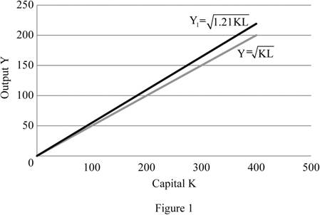
In figure 1, the horizontal axis represents the capital (K) and the vertical axis represents the output (Y). The initial production function
Concept introduction:
Economic growth: The economic growth is the increase in the overall goods and services produced per head in the economy over a specific period of time.
Solow growth rate The Solow growth rate is the rate of economic growth with given flexible price, and the existing real factors of capita, labor and knowledge. The Solow growth rate is an economy’s potential growth rate.
Sub part (c):
Steady state level of output.
Sub part (c):
Explanation of Solution
The new steady state level of output is calculated as follows:
The new steady state level of output is 220 units.
Concept introduction:
Economic growth: The economic growth is the increase in the overall goods and services produced per head in the economy over a specific period of time.
Sub part (d):
The new steady state level of output in the diagram.
Sub part (d):
Explanation of Solution
The new steady state level of output is 220 units which is depicted in the figure 1.
Sub part (e):
Action to gain long lasting benefits from the increase in capital stock.
Sub part (e):
Explanation of Solution
The initial production function is algebraically represented as follows:
Squaring both sides,
And solving for K, we get
Substitute K into the steady-state condition
And solve for Y by multiplying L and dividing by
Similarly, the new production function can be algebraically represented as follows:
Substitute K into the steady-state condition
And solve for Y by multiplying L and dividing by
Equating (1) in (2) we get
Substituting the values in equation (3) we get
Further, the percentage change in the output is depicted as follows:
This implies the steady-state level of output will grow by 21% per cent in the long run.
Concept introduction:
Production function: It is the relationship between the inputs employed by a firm and the maximum output the firm can produce with those inputs.
Sub part (f):
Output per worker.
Sub part (f):
Explanation of Solution
The output per worker in the initial steady state is calculated as follows:
The output per worker in the initial steady state is 2 units per labor.
The output per worker in the short run is calculated as follows:
The output per worker in short run is 1.82 units per labor.
The output per worker in the initial steady state is calculated as follows:
The output per worker in the long run is 2 units per labor.
Sub part (g):
New immigration policy and its effect.
Sub part (g):
Explanation of Solution
The citizens of the country are neither made worse off nor better off in the long run by a new immigration policy. This is because the new long-run level of output per worker compare with the initial level of output per worker remains unchanged which is 2 units per labor. This is unlike the short run effect which has lower output per worker. In the long run, the steady output level is determined largely by the
Concept introduction:
Depreciation: Depreciation is the process of decreasing the value of an asset over time especially due to wear and tear.
Investment: The investment is the money invests in terms of assets and building by the individual for the future consumption and profit making.
Sub part (h):
New steady state level of capital.
Sub part (h):
Explanation of Solution
The new steady state level of capital is calculated as follows
We know
Also
Equating all these we get,
Substituting the values we get
Thus the new steady state level of capital is 484, so that
Want to see more full solutions like this?
Chapter 8 Solutions
EBK MODERN PRINCIPLES OF MICROECONOMICS

- Your marketing department has identified the following customer demographics in the following table. Construct a demand curve and determine the profit maximizing price as well as the expected profit if MC=$1. The number of customers in the target population is 10,000. Use the following demand data: Group Value Frequency Baby boomers $5 20% Generation X $4 10% Generation Y $3 10% `Tweeners $2 10% Seniors $2 10% Others $0 40%arrow_forwardYour marketing department has identified the following customer demographics in the following table. Construct a demand curve and determine the profit maximizing price as well as the expected profit if MC=$1. The number of customers in the target population is 10,000. Group Value Frequency Baby boomers $5 20% Generation X $4 10% Generation Y $3 10% `Tweeners $2 10% Seniors $2 10% Others $0 40% ur marketing department has identified the following customer demographics in the following table. Construct a demand curve and determine the profit maximizing price as well as the expected profit if MC=$1. The number of customers in the target population is 10,000.arrow_forwardTest Preparation QUESTION 2 [20] 2.1 Body Mass Index (BMI) is a summary measure of relative health. It is calculated by dividing an individual's weight (in kilograms) by the square of their height (in meters). A small sample was drawn from the population of UWC students to determine the effect of exercise on BMI score. Given the following table, find the constant and slope parameters of the sample regression function of BMI = f(Weekly exercise hours). Interpret the two estimated parameter values. X (Weekly exercise hours) Y (Body-Mass index) QUESTION 3 2 4 6 8 10 12 41 38 33 27 23 19 Derek investigates the relationship between the days (per year) absent from work (ABSENT) and the number of years taken for the worker to be promoted (PROMOTION). He interviewed a sample of 22 employees in Cape Town to obtain information on ABSENT (X) and PROMOTION (Y), and derived the following: ΣΧ ΣΥ 341 ΣΧΥ 176 ΣΧ 1187 1012 3.1 By using the OLS method, prove that the constant and slope parameters of the…arrow_forward
- QUESTION 2 2.1 [30] Mariana, a researcher at the World Health Organisation (WHO), collects information on weekly study hours (HOURS) and blood pressure level when writing a test (BLOOD) from a sample of university students across the country, before running the regression BLOOD = f(STUDY). She collects data from 5 students as listed below: X (STUDY) 2 Y (BLOOD) 4 6 8 10 141 138 133 127 123 2.1.1 By using the OLS method and the information above derive the values for parameters B1 and B2. 2.1.2 Derive the RSS (sum of squares for the residuals). 2.1.3 Hence, calculate ô 2.2 2.3 (6) (3) Further, she replicates her study and collects data from 122 students from a rival university. She derives the residuals followed by computing skewness (S) equals -1.25 and kurtosis (K) equals 8.25 for the rival university data. Conduct the Jacque-Bera test of normality at a = 0.05. (5) Upon tasked with deriving estimates of ẞ1, B2, 82 and the standard errors (SE) of ẞ1 and B₂ for the replicated data.…arrow_forwardIf you were put in charge of ensuring that the mining industry in canada becomes more sustainable over the course of the next decade (2025-2035), how would you approach this? Come up with (at least) one resolution for each of the 4 major types of conflict: social, environmental, economic, and politicalarrow_forwardHow is the mining industry related to other Canadian labour industries? Choose one other industry, (I chose Forestry)and describe how it is related to the mining industry. How do the two industries work together? Do they ever conflict, or do they work well together?arrow_forward
- What is the primary, secondary, tertiary, and quaternary levels of mining in Canada For each level, describe what types of careers are the most common, and describe what stage your industry’s main resource is in during that stagearrow_forwardHow does the mining industry in canada contribute to the Canadian economy? Describe why your industry is so important to the Canadian economy What would happen if your industry disappeared, or suffered significant layoffs?arrow_forwardWhat is already being done to make mining in canada more sustainable? What efforts are being made in order to make mining more sustainable?arrow_forward
- What are the environmental challenges the canadian mining industry face? Discuss current challenges that mining faces with regard to the environmentarrow_forwardWhat sustainability efforts have been put forth in the mining industry in canada Are your industry’s resources renewable or non-renewable? How do you know? Describe your industry’s reclamation processarrow_forwardHow does oligopolies practice non-price competition in South Africa?arrow_forward

 Principles of Economics (12th Edition)EconomicsISBN:9780134078779Author:Karl E. Case, Ray C. Fair, Sharon E. OsterPublisher:PEARSON
 Engineering Economy (17th Edition)EconomicsISBN:9780134870069Author:William G. Sullivan, Elin M. Wicks, C. Patrick KoellingPublisher:PEARSON
 Principles of Economics (MindTap Course List)EconomicsISBN:9781305585126Author:N. Gregory MankiwPublisher:Cengage Learning
 Managerial Economics: A Problem Solving ApproachEconomicsISBN:9781337106665Author:Luke M. Froeb, Brian T. McCann, Michael R. Ward, Mike ShorPublisher:Cengage Learning
 Managerial Economics & Business Strategy (Mcgraw-...EconomicsISBN:9781259290619Author:Michael Baye, Jeff PrincePublisher:McGraw-Hill Education