
Sub part (a):
Steady state level of output.
Sub part (a):
Explanation of Solution
The steady state level of output is calculated as follows:
The steady state level of output is 200 units.
Concept introduction:
Sub part (b):
Solow diagram to show short run impact.
Sub part (b):
Explanation of Solution
Figure 1 depicts Solow diagram which shows the short run impact of a 21% increase in the amount of labor available.
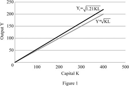
In figure 1, the horizontal axis represents the capital (K) and the vertical axis represents the output (Y). The initial production function
Concept introduction:
Economic growth: The economic growth is the increase in the overall goods and services produced per head in the economy over a specific period of time.
Solow growth rate The Solow growth rate is the rate of economic growth with given flexible price, and the existing real factors of capita, labor and knowledge. The Solow growth rate is an economy’s potential growth rate.
Sub part (c):
Steady state level of output.
Sub part (c):
Explanation of Solution
The new steady state level of output is calculated as follows:
The new steady state level of output is 220 units.
Concept introduction:
Economic growth: The economic growth is the increase in the overall goods and services produced per head in the economy over a specific period of time.
Sub part (d):
The new steady state level of output in the diagram.
Sub part (d):
Explanation of Solution
The new steady state level of output is 220 units which is depicted in the figure 1.
Sub part (e):
Action to gain long lasting benefits from the increase in capital stock.
Sub part (e):
Explanation of Solution
The initial production function is algebraically represented as follows:
Squaring both sides,
And solving for K, we get
Substitute K into the steady-state condition
And solve for Y by multiplying L and dividing by
Similarly, the new production function can be algebraically represented as follows:
Substitute K into the steady-state condition
And solve for Y by multiplying L and dividing by
Equating (1) in (2) we get
Substituting the values in equation (3) we get
Further, the percentage change in the output is depicted as follows:
This implies the steady-state level of output will grow by 21% per cent in the long run.
Concept introduction:
Production function: It is the relationship between the inputs employed by a firm and the maximum output the firm can produce with those inputs.
Sub part (f):
Output per worker.
Sub part (f):
Explanation of Solution
The output per worker in the initial steady state is calculated as follows:
The output per worker in the initial steady state is 2 units per labor.
The output per worker in the short run is calculated as follows:
The output per worker in short run is 1.82 units per labor.
The output per worker in the initial steady state is calculated as follows:
The output per worker in the long run is 2 units per labor.
Sub part (g):
New immigration policy and its effect.
Sub part (g):
Explanation of Solution
The citizens of the country are neither made worse off nor better off in the long run by a new immigration policy. This is because the new long-run level of output per worker compare with the initial level of output per worker remains unchanged which is 2 units per labor. This is unlike the short run effect which has lower output per worker. In the long run, the steady output level is determined largely by the
Concept introduction:
Depreciation: Depreciation is the process of decreasing the value of an asset over time especially due to wear and tear.
Investment: The investment is the money invests in terms of assets and building by the individual for the future consumption and profit making.
Sub part (h):
New steady state level of capital.
Sub part (h):
Explanation of Solution
The new steady state level of capital is calculated as follows
We know
Also
Equating all these we get,
Substituting the values we get
Thus the new steady state level of capital is 484, so that
Want to see more full solutions like this?
Chapter 8 Solutions
EBK MODERN PRINCIPLES OF MICROECONOMICS

- If the US Federal Reserve increases interests on reserves, how will that change the original equilibrium shown in the graph? Euros par US alar 1.10 1.00 0.90- E 0.80- 0.70 0.60 0.50 0.40- 0.30 0.20 47 48 49 50 51 52 53 54 55 56 Quantity of US Dollars traded for Euros (trillions/day) It will increase the demand for Dollars and decrease the supply, so the exchange rate decreases, and the quantity traded increases. O It will decrease the demand for Dollars and increase the supply, so the exchange rate decreases and the impact on the quantity traded is unknown. O It will increase the demand for Dollars and decrease the supply, so the exchange rate increases and the impact on the quantity traded is unknown O It will decrease the demand for Dollars and increase the supply, so the exchange rate decreases, and the quantity traded increases. Question 22 5 ptsarrow_forward1. Based on the video, answer the following questions. • What are the 5 key characteristics that differentiate perfect competition from monopoly? Based on the video. • How does the number of sellers in a market influence the type of market structure? Based on the video. • In what ways does product differentiation play a role in monopolistic competition? Based on the video. • How do barriers to entry affect the level of competition in an oligopoly? Based on the video. • Why might firms in an oligopolistic market engage in non-price competition rather than price wars? Based on the video. Reference video: https://youtu.be/Qrr-IGR1kvE?si=h4q2F1JFNoCI36TVarrow_forward1. Answer the following questions based on the reference video below: • What are the 5 key characteristics that differentiate perfect competition from monopoly? • How does the number of sellers in a market influence the type of market structure? • In what ways does product differentiation play a role in monopolistic competition? • How do barriers to entry affect the level of competition in an oligopoly? • Why might firms in an oligopolistic market engage in non-price competition rather than price wars? Discuss. Reference video: https://youtu.be/Qrr-IGR1kvE?si=h4q2F1JFNoCI36TVarrow_forward
- Explain the importance of differential calculus within economics and business analysis. Provide three refernces with your answer. They can be from websites or a journals.arrow_forwardAnalyze the graph below, showing the Gross Federal Debt as a percentage of GDP for the United States (1939-2019). Which of the following is correct? FRED Gross Federal Debt as Percent of Gross Domestic Product Percent of GDP 120 110 100 60 50 40 90 30 1940 1950 1960 1970 Shaded areas indicate US recessions 1980 1990 2000 2010 1000 Sources: OMD, St. Louis Fed myfred/g/U In 2019, the Federal Government of the United States had an accumulated debt/GDP higher than 100%, meaning that the amount of debt accumulated over time is higher than the value of all goods and services produced in that year. The debt/GDP is always positive during this period, so the Federal Government of the United States incurred in budget deficits every year since 1939. From the mid-40s until the mid-70s, the debt/DGP was decreasing, meaning that the Federal Government of the United States was running a budget surplus every year during those three decades. During the second half of the 1970s, the Federal Government…arrow_forwardAn imaginary country estimates that their economy can be approximated by the AD/AS model below. How can this government act to move the equilibrium to potential GDP? LRAS Price Level P Y Real GDP E SRAS AD The AD/AS model shows that a contractionary fiscal policy is suitable, but the choice of increasing taxes, decreasing government expenditure or doing both simultaneously is mostly political The AD/AS model shows that increasing taxes is the best fiscal policy available. The AD/AS model shows that decreasing government expenditure is the best fiscal policy available. The AD/AS model shows that an expansionary fiscal policy capable of shifting the AD curve to the potential GDP level would decrease Real GDP but increase inflationary pressuresarrow_forward
- Question 1 Coursology Consider the four policies bellow. Classify them as either fiscal or monetary policy: I. The United States Government promoting tax cuts for small businesses to prevent a wave of bankruptcies during the COVID-19 pandemic II. The Congress approving a higher budget for the Affordable Health Care Act (also known as Obamacare) III. The Federal Reserve increasing the required reserves for commercial banks aiming to control the rise of inflation IV. President Joe Biden approving a new round of stimulus checks for households I. fiscal, II. fiscal, III. monetary, IV. fiscal I. fiscal, II. monetary, III. monetary, IV. monetary I. monetary, II. fiscal, III. fiscal, IV. fiscal I. monetary, II. monetary, III. fiscal, IV. monetaryarrow_forwardConsider the following supply and demand schedule of wooden tables.a. Draw the corresponding graphs for supply and demand.b. Using the data, obtain the corresponding supply and demand functions. c. Find the market-clearing price and quantity. Price (Thousand s USD Supply Demand 2 96 1104 196 1906 296 2708 396 35010 496 43012 596 51014 696 59016 796 67018 896 75020…arrow_forwardConsider a firm with the following production function Q=5000L-2L2.a. Find the maximum production level.b. How many units of labour are needed at that point. c. Obtain the function of marginal product of labour (MRL) d. Graph the production function and the MRL.arrow_forward
- Exercise 4A firm has the following total cost function TC=100q-5q2+0.5q3. Find the average cost function.arrow_forwardA firm has the following demand function P=200 − 2Q and the average costof AC= 100/Q + 3Q −20.a. Find the profit function. b. Estimate the marginal cost function. c. Obtain the production that maximizes the profit. d. Evaluate the average cost and the marginal cost at the maximising production level.arrow_forwardRubber: Initial investment: $159,000 Annual cost: $36,000 Annual revenue: $101,000 Salvage value: $12,000 Useful life: 10 years Using the cotermination assumptions, a study period of 6 years, and a MARR of 9%, what is the present worth of the rubber alternative? Assume that the rubber alternative's equipment has a market value of $18,000 at the end of Year 6.arrow_forward

 Principles of Economics (12th Edition)EconomicsISBN:9780134078779Author:Karl E. Case, Ray C. Fair, Sharon E. OsterPublisher:PEARSON
 Engineering Economy (17th Edition)EconomicsISBN:9780134870069Author:William G. Sullivan, Elin M. Wicks, C. Patrick KoellingPublisher:PEARSON
 Principles of Economics (MindTap Course List)EconomicsISBN:9781305585126Author:N. Gregory MankiwPublisher:Cengage Learning
 Managerial Economics: A Problem Solving ApproachEconomicsISBN:9781337106665Author:Luke M. Froeb, Brian T. McCann, Michael R. Ward, Mike ShorPublisher:Cengage Learning
 Managerial Economics & Business Strategy (Mcgraw-...EconomicsISBN:9781259290619Author:Michael Baye, Jeff PrincePublisher:McGraw-Hill Education