
Concept explainers
Videos
For Exercises 1 through 20, perform each of the following steps.
a. State the hypotheses and identify the claim.
b. Find the critical value(s).
c. Compute the test value.
d. Make the decision.
e. Summarize the results.
Use the traditional method of hypothesis testing unless otherwise specified.
1. Lifetime of $1 Bills The average lifetime of circulated $1 bills is 18 months. A researcher believes that the average lifetime is not 18 months. He researched the lifetime of 50 $1 bills and found the average lifetime was 18.8 months. The population standard deviation is 2.8 months. At α = 0.02, can it be concluded that the average lifetime of a circulated $1 bill differs from 18 months?
a.
To state: The null and alternative hypotheses and identify the claim.
Answer to Problem 8.2.1RE
Null hypothesis:
Alternative hypothesis:
The claim is “the average lifetime of circulated $1 bills is not 18 months”.
Explanation of Solution
Given info:
A sample of 50 $1 bills selected and found the average lifetime was 18.8 months. The population standard deviation is 2.8 months.
Justification:
Here, the claim is that the average lifetime of circulated $1 bills is not 18 months. This can be written as
The test hypotheses are given below:
Null hypothesis: The average lifetime of circulated $1 bills is 18 months
Alternative hypothesis (claim): The average lifetime of circulated $1 bills is not 18 months.
b.
To find: The critical values.
Answer to Problem 8.2.1RE
The critical value is ±2.326.
Explanation of Solution
Calculation:
Software Procedure:
Step-by-step procedure to obtain the critical value using the MINITAB software:
- Choose Graph > Probability Distribution Plot choose View Probability > OK.
- From Distribution, choose ‘Normal’ distribution.
- Click the Shaded Area tab.
- Choose Probability Value and Both Tail for the region of the curve to shade.
- Enter the Probability value as 0.02.
- Click OK.
Output using the MINITAB software is given below:
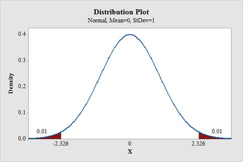
From the output, the critical value is ±2.326.
c.
To find: The test value.
Answer to Problem 8.2.1RE
The test value is 2.02.
Explanation of Solution
Calculation:
Software Procedure:
Step-by-step procedure to obtain the test value using the MINITAB software:
- Choose Stat > Basic Statistics > 1-Sample Z.
- In Summarized data, enter the sample size as 50 and mean as 18.8.
- In Standard deviation, enter 2.8.
- In Perform hypothesis test, enter the test mean as 18.
- Check Options; enter Confidence level as 98%.
- Choose not equal in alternative.
- Click OK.
Output using the MINITAB software is given below:
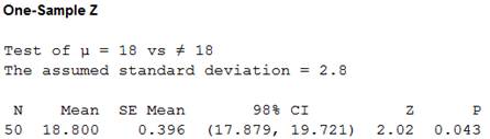
From the output, the test value is 2.02.
d.
To make: The decision.
Answer to Problem 8.2.1RE
The decision is “fail to reject the null hypothesis”.
Explanation of Solution
Calculation:
Software Procedure:
Step-by-step procedure to indicate the appropriate area and critical value using the MINITAB software:
- Choose Graph > Probability Distribution Plot choose View Probability > OK.
- From Distribution, choose ‘Normal’ distribution.
- Click the Shaded Area tab.
- Choose Probability Value and Both Tail for the region of the curve to shade.
- Enter the Probability value as 0.02.
- Enter 2.02 under show reference lines at X values.
- Click OK.
Output using the MINITAB software is given below:
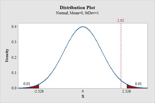
From the output, it can be observed that the test statistic value do not falls in the critical region. Therefore, the null hypothesis is not rejected.
e.
To summarize: The result.
Answer to Problem 8.2.1RE
The conclusion is that, there is no enough evidence to support the claim that the average lifetime of circulated $1 bills is not 18 months.
Explanation of Solution
Justification:
From part d, the null hypothesis is not rejected. Therefore, there is no enough evidence to support the claim that the average lifetime of circulated $1 bills is not 18 months.
Want to see more full solutions like this?
Chapter 8 Solutions
ELEMENTARY STATISTICS: STEP BY STEP- ALE


- The U.S. Postal Service will ship a Priority Mail® Large Flat Rate Box (12" 3 12" 3 5½") any where in the United States for a fixed price, regardless of weight. The weights (ounces) of 20 ran domly chosen boxes are shown below. (a) Make a stem-and-leaf diagram. (b) Make a histogram. (c) Describe the shape of the distribution. Weights 72 86 28 67 64 65 45 86 31 32 39 92 90 91 84 62 80 74 63 86arrow_forward(a) What is a bimodal histogram? (b) Explain the difference between left-skewed, symmetric, and right-skewed histograms. (c) What is an outlierarrow_forward(a) Test the hypothesis. Consider the hypothesis test Ho = : against H₁o < 02. Suppose that the sample sizes aren₁ = 7 and n₂ = 13 and that $² = 22.4 and $22 = 28.2. Use α = 0.05. Ho is not ✓ rejected. 9-9 IV (b) Find a 95% confidence interval on of 102. Round your answer to two decimal places (e.g. 98.76).arrow_forward
- Let us suppose we have some article reported on a study of potential sources of injury to equine veterinarians conducted at a university veterinary hospital. Forces on the hand were measured for several common activities that veterinarians engage in when examining or treating horses. We will consider the forces on the hands for two tasks, lifting and using ultrasound. Assume that both sample sizes are 6, the sample mean force for lifting was 6.2 pounds with standard deviation 1.5 pounds, and the sample mean force for using ultrasound was 6.4 pounds with standard deviation 0.3 pounds. Assume that the standard deviations are known. Suppose that you wanted to detect a true difference in mean force of 0.25 pounds on the hands for these two activities. Under the null hypothesis, 40 = 0. What level of type II error would you recommend here? Round your answer to four decimal places (e.g. 98.7654). Use a = 0.05. β = i What sample size would be required? Assume the sample sizes are to be equal.…arrow_forward= Consider the hypothesis test Ho: μ₁ = μ₂ against H₁ μ₁ μ2. Suppose that sample sizes are n₁ = 15 and n₂ = 15, that x1 = 4.7 and X2 = 7.8 and that s² = 4 and s² = 6.26. Assume that o and that the data are drawn from normal distributions. Use απ 0.05. (a) Test the hypothesis and find the P-value. (b) What is the power of the test in part (a) for a true difference in means of 3? (c) Assuming equal sample sizes, what sample size should be used to obtain ẞ = 0.05 if the true difference in means is - 2? Assume that α = 0.05. (a) The null hypothesis is 98.7654). rejected. The P-value is 0.0008 (b) The power is 0.94 . Round your answer to four decimal places (e.g. Round your answer to two decimal places (e.g. 98.76). (c) n₁ = n2 = 1 . Round your answer to the nearest integer.arrow_forwardConsider the hypothesis test Ho: = 622 against H₁: 6 > 62. Suppose that the sample sizes are n₁ = 20 and n₂ = 8, and that = 4.5; s=2.3. Use a = 0.01. (a) Test the hypothesis. Round your answers to two decimal places (e.g. 98.76). The test statistic is fo = i The critical value is f = Conclusion: i the null hypothesis at a = 0.01. (b) Construct the confidence interval on 02/022 which can be used to test the hypothesis: (Round your answer to two decimal places (e.g. 98.76).) iarrow_forward
- 2011 listing by carmax of the ages and prices of various corollas in a ceratin regionarrow_forwardس 11/ أ . اذا كانت 1 + x) = 2 x 3 + 2 x 2 + x) هي متعددة حدود محسوبة باستخدام طريقة الفروقات المنتهية (finite differences) من جدول البيانات التالي للدالة (f(x . احسب قيمة . ( 2 درجة ) xi k=0 k=1 k=2 k=3 0 3 1 2 2 2 3 αarrow_forward1. Differentiate between discrete and continuous random variables, providing examples for each type. 2. Consider a discrete random variable representing the number of patients visiting a clinic each day. The probabilities for the number of visits are as follows: 0 visits: P(0) = 0.2 1 visit: P(1) = 0.3 2 visits: P(2) = 0.5 Using this information, calculate the expected value (mean) of the number of patient visits per day. Show all your workings clearly. Rubric to follow Definition of Random variables ( clearly and accurately differentiate between discrete and continuous random variables with appropriate examples for each) Identification of discrete random variable (correctly identifies "number of patient visits" as a discrete random variable and explains reasoning clearly.) Calculation of probabilities (uses the probabilities correctly in the calculation, showing all steps clearly and logically) Expected value calculation (calculate the expected value (mean)…arrow_forward
- if the b coloumn of a z table disappeared what would be used to determine b column probabilitiesarrow_forwardConstruct a model of population flow between metropolitan and nonmetropolitan areas of a given country, given that their respective populations in 2015 were 263 million and 45 million. The probabilities are given by the following matrix. (from) (to) metro nonmetro 0.99 0.02 metro 0.01 0.98 nonmetro Predict the population distributions of metropolitan and nonmetropolitan areas for the years 2016 through 2020 (in millions, to four decimal places). (Let x, through x5 represent the years 2016 through 2020, respectively.) x₁ = x2 X3 261.27 46.73 11 259.59 48.41 11 257.96 50.04 11 256.39 51.61 11 tarrow_forwardIf the average price of a new one family home is $246,300 with a standard deviation of $15,000 find the minimum and maximum prices of the houses that a contractor will build to satisfy 88% of the market valuearrow_forward
 Glencoe Algebra 1, Student Edition, 9780079039897...AlgebraISBN:9780079039897Author:CarterPublisher:McGraw Hill