Chapter 8, Problem 49P

1.

To determine

Compute quarterly forecast by selecting two data point from part (1) using high-low method.

Explanation of Solution

High-low method:

The graph in part (1) shows that high and low points are last and second data points, so these points develop the estimate of high-low.

Calculate the variable cost.

$\begin{array}{c}\text{Variable cost}=\frac{\left(\begin{array}{l}\text{Return expense of 4th quarter 2018}\\ \text{Return expense of 2nd quarter 2016}\end{array}\right)}{\left(\begin{array}{l}\text{Last data point}\\ -\text{Second data point}\end{array}\right)}\\ =\frac{\$14,600-\$11,300}{12-2}\\ =\$330\end{array}$

Calculate the fixed cost.

$\begin{array}{c}\text{Fixed cost}=\left(\begin{array}{l}\text{Return expense of 2nd quarter 2016}\\ -\left(\text{Variable cost}\times \text{Second data point}\right)\end{array}\right)\\ =\$11,300-\left(\$330\times 2\right)\\ =\$10,640\end{array}$

Compute quarterly prediction for the year 2019.

2019 Quarter	Return Expenses
13	$14,930
14	$15,260
15	$15,590
16	$15,920

Table (1)

Note: Shown below is the formula to compute quarterly prediction.

$\text{Quarterly prediction}=\left(\begin{array}{l}2019\text{ quarter}\\ \times \text{Variable cost}\\ \text{+Fixed cost}\end{array}\right)$

These predictions do not take into account the seasonal variation as shown in the data, it is always useful to take into consideration the results for a regression analysis as shown in part (3).

Compute the quarterly forecast for 2019 using the results of a regression analysis. Calculate the result of regression analysis and necessary changes to improve the model.

Regression one:

Regression Statistics
Multiple R	0.439734422
R Square	0.193366362
Adjusted R Square	0.112702998
Standard Error	974.8928577
Observations	12

Table (2)

ANOVA
	df	SS	MS	F	Significance F
Regression	1	2278339.161	2278339	2.397202	0.152593037
Residual	10	9504160.839	950416.1
Total	11	11782500

Table (3)

Table (4)

Regression Predictions
Intercept	$11,855
Coefficient	$126.22

Table (5)

Quarterly Predictions
13	$13,496
14	$13,622
15	$13,748
16	$13,875

Table (6)

Note: Shown below is to compute rent expense.

$\text{Rent expense}=\left(\begin{array}{l}\text{Intercept in regression 1}\\ +\left(\begin{array}{l}\text{Quarter of co-efficients}\\ \times \text{Quarter number}\end{array}\right)\end{array}\right)$

Predicted expense for next four quarter using regression analysis:

Quarter	Regression prediction
13	$\left(\$11,855+\left(13\times \$126.2238\right)\right)$	13,495.45
14	$\left(\$11,855+\left(14\times \$126.2238\right)\right)$	13,621.68
15	$\left(\$11,855+\left(15\times \$126.2238\right)\right)$	13,747.90
16	$\left(\$11,855+\left(16\times \$126.2238\right)\right)$	13,874.13

Table (7)

This shows how the regression model’s prediction differ from that of high-low method.

The above regression one has relatively low R-Squared (0.19) and low t-value for the independent variable, a revision of the regression model is considered. Since, there is visible seasonality in the data, by adding dummy variable it is possible to improve on the regression model with 1s in the periods 4, 8, and 12, and 0s in the left-over periods. For the dummy variable the below given regression analysis indications a much higher R-Squared, improved SE and a substantial t-value.

Regression 2:

Regression Statistics
Multiple R	0.873681599
R Square	0.763319537
Adjusted R Square	0.710723879
Standard Error	556.6454641
Observations	12

Table (8)

ANOVA
	df	SS	MS	F	Significance F
Regression	2	8993812.445	4496906.223	14.51297616	0.00152662
Residual	9	2788687.555	309854.1728
Total	11	11782500

Table (9)

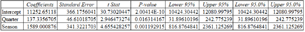
Table (10)

Equation for the above regression are:

$\text{Expenses}=\left(\begin{array}{l}\text{\$11,252}\text{.65118}\\ \text{+}\left(\begin{array}{l}\$1,589,00876\\ \times \text{Dummy variable for season}\end{array}\right)\\ +\left(\$137.33567\times \text{Quarter number}\right)\end{array}\right)$

Regression Predictions
Intercept	$11,252.65
Coefficient Qtr.	$137.34
Coefficient Season	$1,589

Table (11)

The regression prediction for the revised regression:

Quarterly Predictions
13	$14,627
14	$13,175
15	$13,313
16	$15,039

Table (12)

The management accountant should depend on the above shown prediction because the second regression has better statistical measures.

2.

To determine

Explain how the analysis of costs change, if L Incorporation produces its products in multiple global production facilities to serve the global market.

Explanation of Solution

If L Incorporation produces its products in multiple global production facilities, then the expenses incurred from returns has to be studied by the production facility. Due to various equipment used in manufacturing the DVD players, the cost incurred are likely to differ among the production facility.