
Concept explainers
Videos
a.
To find: The equation of the least-squares line for predicting a neuron's call response from its pure tone response.
To construct: The
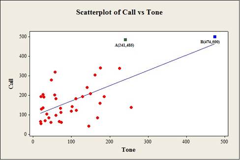
To construct: The scatter plot with the point A which is the largest residual (either positive or negative) and also the point B that is an outlier in the x direction.
a.
Answer to Problem 7.56SE
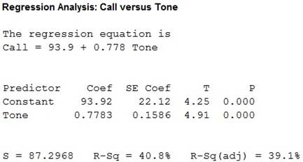
The equation of the least-squares line for predicting a neuron's call response from its pure tone response is
Output using the MINITAB software is given below:
Output with marked point A and B using the MINITAB software is given below:
Explanation of Solution
The given data shows the pure-tone response and monkey call response values.
Calculation:
Software procedure:
Step by step procedure to find the equation of the least-squares line by using the MINITAB software:
- Choose Stat > Regression > Regression.
- In Responses, enter the column of Call.
- In Predictors, enter the column of Tone.
- Click OK.
Output using the MINITAB software is given below:
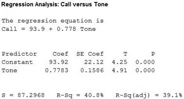
From the MINITAB output, it is clear that the regression equation is
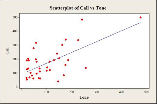
Scatterplot:
Software procedure:
Step by step procedure to construct the scatter plots using the MINITAB software:
- Choose Graph > Scatter plot.
- Choose with regression and groups, and then click OK.
- Under Y variables, enter a column of Call.
- Under X variables, enter a column of Tone.
- Click OK.
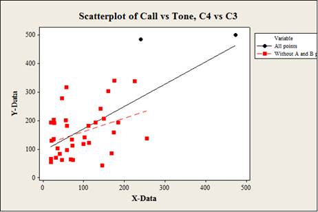
From the scatterplot, it is observed that the plot shows no distinct pattern. Also, the x (pure-tone response) values increase then the corresponding y (monkey call response) values increase. Also, the points are moderately scattered. Thus, there is moderately
Also, from the scatterplot, it is observed that the largest residual is marked as point A(241,485) and also the outlier in the x direction point is marked as B(474,500).
b.
To explain: The influences of the points A and B for the
b.
Answer to Problem 7.56SE
The outlier and residual is removed then the correlation decreases.
Explanation of Solution
Calculation:
Correlation: With points A and B
Step by step procedure to obtain the correlation using the MINITAB software:
- Select Stat > Basic Statistics > Correlation.
- In Variables, select X, and Y from the box on the left.
- Click OK.
Output using the MINITAB software is given below:
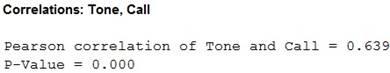
From the output, the correlation with points A and B is 0.639.
Correlation: Without points A and B.
Step by step procedure to obtain the correlation using the MINITAB software:
- Select Stat > Basic Statistics > Correlation.
- In Variables, select X, and Y from the box on the left.
- Click OK.
Output using the MINITAB software is given below:
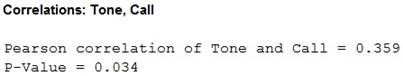
From the output, the correlation without points A and B is 0.359.
The correlation with points A and B is 0.639 and the correlation without points A and B is 0.359. Also, from the scatterplot in part (a), it is observed that the outlier and residual deviate from linear pattern of the other points.
Thus, it can be concluded that if the outlier and residual are removed then the correlation decreases. Thus, the outlier and residual influence the correlation.
c.
To explain: The influences of the points A and B for the least-squares line.
c.
Answer to Problem 7.56SE
The effect of the outlier and residual influences on the line is small.
Explanation of Solution
Calculation:
Regression: With Fidelity Gold Fund.
Step by step procedure to obtain the regression using the MINITAB software:
- Choose Stat > Regression > Regression.
- In Responses, enter the column of y.
- In Predictors, enter the column of x.
- Click OK.
Output using the MINITAB software is given below:
From the output, the least-squares line for predicting y from x with points A and B is
Regression: Without points A and B.
Step by step procedure to obtain the regression using the MINITAB software:
- Choose Stat > Regression > Regression.
- In Responses, enter the column of y.
- In Predictors, enter the column of x.
- Click OK.
Output using the MINITAB software is given below:

From the output, the least-squares line for predicting y from x without points A and B is
Scatter plot:
Step by step procedure to construct the scatter plots with two regression line using the MINITAB software:
- Choose Graph > Scatter plot.
- Choose with regression and groups, and then click OK.
- Under Y variables, enter a column of Y.
- Under X variables, enter a column of X.
- Click OK.
Output using the MINITAB software is given below:
Observation:
From the scatterplot with two regression lines, it is observed that the horizontal axis represents the pure-tone response values and vertical axis represents the monkey call response values. Also, the regression line with all points is marked with solid line and the regression line without points A and B is marked with dashed line.
Also, it is observed that the effect of the points A and B on the line is small. Hence, the residual and outlier was not particularly extreme in the pure-tone response.
Thus, it can be concluded that the outlier and residual do not influence the least-square regression line.
Want to see more full solutions like this?
Chapter 7 Solutions
EBK THE BASIC PRACTICE OF STATISTICS


- Name Harvard University California Institute of Technology Massachusetts Institute of Technology Stanford University Princeton University University of Cambridge University of Oxford University of California, Berkeley Imperial College London Yale University University of California, Los Angeles University of Chicago Johns Hopkins University Cornell University ETH Zurich University of Michigan University of Toronto Columbia University University of Pennsylvania Carnegie Mellon University University of Hong Kong University College London University of Washington Duke University Northwestern University University of Tokyo Georgia Institute of Technology Pohang University of Science and Technology University of California, Santa Barbara University of British Columbia University of North Carolina at Chapel Hill University of California, San Diego University of Illinois at Urbana-Champaign National University of Singapore…arrow_forwardA company found that the daily sales revenue of its flagship product follows a normal distribution with a mean of $4500 and a standard deviation of $450. The company defines a "high-sales day" that is, any day with sales exceeding $4800. please provide a step by step on how to get the answers in excel Q: What percentage of days can the company expect to have "high-sales days" or sales greater than $4800? Q: What is the sales revenue threshold for the bottom 10% of days? (please note that 10% refers to the probability/area under bell curve towards the lower tail of bell curve) Provide answers in the yellow cellsarrow_forwardFind the critical value for a left-tailed test using the F distribution with a 0.025, degrees of freedom in the numerator=12, and degrees of freedom in the denominator = 50. A portion of the table of critical values of the F-distribution is provided. Click the icon to view the partial table of critical values of the F-distribution. What is the critical value? (Round to two decimal places as needed.)arrow_forward
- A retail store manager claims that the average daily sales of the store are $1,500. You aim to test whether the actual average daily sales differ significantly from this claimed value. You can provide your answer by inserting a text box and the answer must include: Null hypothesis, Alternative hypothesis, Show answer (output table/summary table), and Conclusion based on the P value. Showing the calculation is a must. If calculation is missing,so please provide a step by step on the answers Numerical answers in the yellow cellsarrow_forwardShow all workarrow_forwardShow all workarrow_forward
 MATLAB: An Introduction with ApplicationsStatisticsISBN:9781119256830Author:Amos GilatPublisher:John Wiley & Sons Inc
 Probability and Statistics for Engineering and th...StatisticsISBN:9781305251809Author:Jay L. DevorePublisher:Cengage Learning
 Statistics for The Behavioral Sciences (MindTap C...StatisticsISBN:9781305504912Author:Frederick J Gravetter, Larry B. WallnauPublisher:Cengage Learning
 Elementary Statistics: Picturing the World (7th E...StatisticsISBN:9780134683416Author:Ron Larson, Betsy FarberPublisher:PEARSON
 The Basic Practice of StatisticsStatisticsISBN:9781319042578Author:David S. Moore, William I. Notz, Michael A. FlignerPublisher:W. H. Freeman
 Introduction to the Practice of StatisticsStatisticsISBN:9781319013387Author:David S. Moore, George P. McCabe, Bruce A. CraigPublisher:W. H. Freeman