
a.
The
a.
Answer to Problem 7.38TY
The scatter plot is shown below,
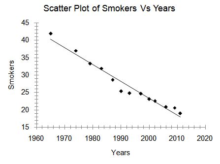
Figure (1)
Explanation of Solution
Given Info:
The percentages of adult smokers in the years between 1965 and 2011 is given below,
| Years | Smokers |
| 1965 | 41.9 |
| 1974 | 37 |
| 1979 | 33.3 |
| 1983 | 31.9 |
| 1987 | 28.6 |
| 1990 | 25.3 |
| 1993 | 24.8 |
| 1997 | 24.6 |
| 2000 | 23.1 |
| 2002 | 22.5 |
| 2006 | 20.8 |
| 2009 | 20.6 |
| 2011 | 19 |
Software Procedure:
Step by step procedure to draw the scatterplot using the Excel:
Steps to draw a scatter plot of the given data are:
- Press [Ctrl]-N for a new workbook.
- Enter the years column A.
- Enter the percent of adult smokers into column B.
- Select Add ins then Megastats.
- Select
Correlation/Regression and under that select scatter plot. - Select the column 1 in horizontal axis and column 2 in vertical axis.
- Tick the plot linear regression line and press Ok.
Output using the Excel is given below:
Observation:
The scatter plot shows that, the number of smokers’ decreases as the year’s increases.
b.
The direction, form, and strength of the relationship between percent of smokers and year. Whether there are any outliers.
b.
Explanation of Solution
From the scatterplot, it is clear that the value of smokers decreases with increase in number of year that means there is a linear relationship between smokers and years and number of smokers decreases with increase in year so, relationship is negative.
Thus, there is a strong negative linear relationship between the smokers and the year and there are no outliers.
c.
The least squares regression line that predicts percent of smokers from year and add the line to the scatter plot.
c.
Answer to Problem 7.38TY
The equation of the least square regression line is
Explanation of Solution
Given info:
The given values are,
Calculation:
The formula for regression equation is given below,
Where,
The formula to calculate the value of b is,
Substitute
The value of b is
The formula to calculate the value of a is,
Substitute
The value of a is
Substitute
Thus, the equation of the least square regression line is
d.
The decline in smoking per year on an average during this period.
d.
Answer to Problem 7.38TY
The decline in smoking per year on an average during this period is
Explanation of Solution
Calculation:
The equation of the least square regression line is,
The slope of the regression is
The coefficient value for year is
Thus, the decline in smoking per year on an average during this period is
e.
The percentage of the variation of adults who smoke can be explained by linear change over time.
e.
Answer to Problem 7.38TY
The percentage of the variation of adults who smoke can be explained by linear change over time is 96.04%.
Explanation of Solution
Calculation:
The formula to find percentage of the variation of adults who smoke can be explained by linear change over time is given by squared value of r.
Thus, the percentage of the variation of adults who smoke can be explained by linear change over time is 96.04%.
f.
The percentage of smokers in 2020.
f.
Answer to Problem 7.38TY
The predicted percentage of adults that smoke in 2020 is 13.48%.
Explanation of Solution
Calculation:
From part (c) the equation for linear regression is given by,
Where,
- x represents the year.
-
Substitute 2020 for x in the above equation to find the percentage of smokers in 2020.
Thus, the predicted percentage of adults that smoke in 2020 is 13.48%.
g.
The percentage of smokers in 2075. And reason that it is foolishness to use this regression line equation to find the percentage of smokers in 2075.
g.
Answer to Problem 7.38TY
The predicted percentage of adults that smoke in 2075 is 13.48%.
Explanation of Solution
Calculation:
From part (c) the equation for linear regression is given by,
Where,
- x represents the year.
-
Substitute 2075 for x in the above equation to find the percentage of smokers in 2075.
Thus, the predicted percentage of adults that smoke in 2020 is
Clearly, the percentage of smokers came out to be negative in 2075 which is impossible.
Thus, it is foolishness to use this regression line equation to find the percentage of smokers in 2075.
Want to see more full solutions like this?
Chapter 7 Solutions
The Basic Practice of Statistics

- 1. If a firm spends more on advertising, is it likely to increase sales? Data on annual sales (in $100,000s) and advertising expenditures (in $10,000s) were collected for 20 firms in order to estimate the model Sales = Po + B₁Advertising + ε. A portion of the regression results is shown in the accompanying table. Intercept Advertising Standard Coefficients Error t Stat p-value -7.42 1.46 -5.09 7.66E-05 0.42 0.05 8.70 7.26E-08 a. Interpret the estimated slope coefficient. b. What is the sample regression equation? C. Predict the sales for a firm that spends $500,000 annually on advertising.arrow_forwardCan you help me solve problem 38 with steps im stuck.arrow_forwardHow do the samples hold up to the efficiency test? What percentages of the samples pass or fail the test? What would be the likelihood of having the following specific number of efficiency test failures in the next 300 processors tested? 1 failures, 5 failures, 10 failures and 20 failures.arrow_forward
- The battery temperatures are a major concern for us. Can you analyze and describe the sample data? What are the average and median temperatures? How much variability is there in the temperatures? Is there anything that stands out? Our engineers’ assumption is that the temperature data is normally distributed. If that is the case, what would be the likelihood that the Safety Zone temperature will exceed 5.15 degrees? What is the probability that the Safety Zone temperature will be less than 4.65 degrees? What is the actual percentage of samples that exceed 5.25 degrees or are less than 4.75 degrees? Is the manufacturing process producing units with stable Safety Zone temperatures? Can you check if there are any apparent changes in the temperature pattern? Are there any outliers? A closer look at the Z-scores should help you in this regard.arrow_forwardNeed help pleasearrow_forwardPlease conduct a step by step of these statistical tests on separate sheets of Microsoft Excel. If the calculations in Microsoft Excel are incorrect, the null and alternative hypotheses, as well as the conclusions drawn from them, will be meaningless and will not receive any points. 4. One-Way ANOVA: Analyze the customer satisfaction scores across four different product categories to determine if there is a significant difference in means. (Hints: The null can be about maintaining status-quo or no difference among groups) H0 = H1=arrow_forward
- Please conduct a step by step of these statistical tests on separate sheets of Microsoft Excel. If the calculations in Microsoft Excel are incorrect, the null and alternative hypotheses, as well as the conclusions drawn from them, will be meaningless and will not receive any points 2. Two-Sample T-Test: Compare the average sales revenue of two different regions to determine if there is a significant difference. (Hints: The null can be about maintaining status-quo or no difference among groups; if alternative hypothesis is non-directional use the two-tailed p-value from excel file to make a decision about rejecting or not rejecting null) H0 = H1=arrow_forwardPlease conduct a step by step of these statistical tests on separate sheets of Microsoft Excel. If the calculations in Microsoft Excel are incorrect, the null and alternative hypotheses, as well as the conclusions drawn from them, will be meaningless and will not receive any points 3. Paired T-Test: A company implemented a training program to improve employee performance. To evaluate the effectiveness of the program, the company recorded the test scores of 25 employees before and after the training. Determine if the training program is effective in terms of scores of participants before and after the training. (Hints: The null can be about maintaining status-quo or no difference among groups; if alternative hypothesis is non-directional, use the two-tailed p-value from excel file to make a decision about rejecting or not rejecting the null) H0 = H1= Conclusion:arrow_forwardPlease conduct a step by step of these statistical tests on separate sheets of Microsoft Excel. If the calculations in Microsoft Excel are incorrect, the null and alternative hypotheses, as well as the conclusions drawn from them, will be meaningless and will not receive any points. The data for the following questions is provided in Microsoft Excel file on 4 separate sheets. Please conduct these statistical tests on separate sheets of Microsoft Excel. If the calculations in Microsoft Excel are incorrect, the null and alternative hypotheses, as well as the conclusions drawn from them, will be meaningless and will not receive any points. 1. One Sample T-Test: Determine whether the average satisfaction rating of customers for a product is significantly different from a hypothetical mean of 75. (Hints: The null can be about maintaining status-quo or no difference; If your alternative hypothesis is non-directional (e.g., μ≠75), you should use the two-tailed p-value from excel file to…arrow_forward
- Please conduct a step by step of these statistical tests on separate sheets of Microsoft Excel. If the calculations in Microsoft Excel are incorrect, the null and alternative hypotheses, as well as the conclusions drawn from them, will be meaningless and will not receive any points. 1. One Sample T-Test: Determine whether the average satisfaction rating of customers for a product is significantly different from a hypothetical mean of 75. (Hints: The null can be about maintaining status-quo or no difference; If your alternative hypothesis is non-directional (e.g., μ≠75), you should use the two-tailed p-value from excel file to make a decision about rejecting or not rejecting null. If alternative is directional (e.g., μ < 75), you should use the lower-tailed p-value. For alternative hypothesis μ > 75, you should use the upper-tailed p-value.) H0 = H1= Conclusion: The p value from one sample t-test is _______. Since the two-tailed p-value is _______ 2. Two-Sample T-Test:…arrow_forwardPlease conduct a step by step of these statistical tests on separate sheets of Microsoft Excel. If the calculations in Microsoft Excel are incorrect, the null and alternative hypotheses, as well as the conclusions drawn from them, will be meaningless and will not receive any points. What is one sample T-test? Give an example of business application of this test? What is Two-Sample T-Test. Give an example of business application of this test? .What is paired T-test. Give an example of business application of this test? What is one way ANOVA test. Give an example of business application of this test? 1. One Sample T-Test: Determine whether the average satisfaction rating of customers for a product is significantly different from a hypothetical mean of 75. (Hints: The null can be about maintaining status-quo or no difference; If your alternative hypothesis is non-directional (e.g., μ≠75), you should use the two-tailed p-value from excel file to make a decision about rejecting or not…arrow_forwardThe data for the following questions is provided in Microsoft Excel file on 4 separate sheets. Please conduct a step by step of these statistical tests on separate sheets of Microsoft Excel. If the calculations in Microsoft Excel are incorrect, the null and alternative hypotheses, as well as the conclusions drawn from them, will be meaningless and will not receive any points. What is one sample T-test? Give an example of business application of this test? What is Two-Sample T-Test. Give an example of business application of this test? .What is paired T-test. Give an example of business application of this test? What is one way ANOVA test. Give an example of business application of this test? 1. One Sample T-Test: Determine whether the average satisfaction rating of customers for a product is significantly different from a hypothetical mean of 75. (Hints: The null can be about maintaining status-quo or no difference; If your alternative hypothesis is non-directional (e.g., μ≠75), you…arrow_forward
 MATLAB: An Introduction with ApplicationsStatisticsISBN:9781119256830Author:Amos GilatPublisher:John Wiley & Sons Inc
 Probability and Statistics for Engineering and th...StatisticsISBN:9781305251809Author:Jay L. DevorePublisher:Cengage Learning
 Statistics for The Behavioral Sciences (MindTap C...StatisticsISBN:9781305504912Author:Frederick J Gravetter, Larry B. WallnauPublisher:Cengage Learning
 Elementary Statistics: Picturing the World (7th E...StatisticsISBN:9780134683416Author:Ron Larson, Betsy FarberPublisher:PEARSON
 The Basic Practice of StatisticsStatisticsISBN:9781319042578Author:David S. Moore, William I. Notz, Michael A. FlignerPublisher:W. H. Freeman
 Introduction to the Practice of StatisticsStatisticsISBN:9781319013387Author:David S. Moore, George P. McCabe, Bruce A. CraigPublisher:W. H. Freeman