Chapter 7, Problem 13CRP

(a)

To determine

Identify the problem based on the parameter being estimated.

Check the sample mean by using the calculator.

Check the sample standard deviation by using the calculator.

Answer to Problem 13CRP

The problem is categorized as interval for difference in mean based on the parameter being estimated.

Explanation of Solution

Calculation:

The ${\mu }_1$ is the population mean for soil water content from field I and ${\mu }_2$ is the population mean for soil water content from field II. The confidence interval for difference between the means has to be calculated, that is ${\mu }_1-{\mu }_2$. This shows that, the parameter being estimated in the study is ${\mu }_1-{\mu }_2$.

Hence, the problem is categorized as interval for difference in mean based on the parameter being estimated.

Mean and standard deviation for $x_1$:

Use Ti 83 calculator to find the mean and standard deviation as follows:

• Select STAT > Edit > Enter the values of $x_1$ as L1.
• Click $\boxed{2^{\text{nd}}}$ button; STAT; take the arrow to the MATH menu, and then ‘3’ numbered key.
• Click $\boxed{2^{\text{nd}}}$ button; then ‘1’ numbered key to get L1, and close the ‘)’ bracket.
• Click Enter.
• Click $\boxed{2^{\text{nd}}}$ button; STAT; take the arrow to the MATH menu, and then ‘7’ numbered key.
• Click $\boxed{2^{\text{nd}}}$ button; then ‘1’ numbered key to get L1, and close the ‘)’ bracket.
• Click Enter.

Output using Ti 83 calculator is given below:

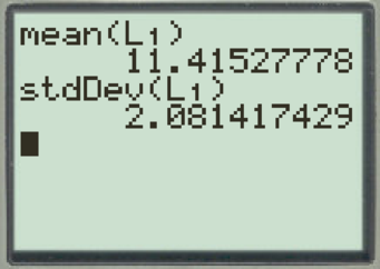
From the Ti 83 calculator output, the mean value is 11.42, and standard deviation value is 2.08.

Mean and standard deviation for $x_2$:

Use Ti 83 calculator to find the mean and standard deviation as follows:

• Select STAT > Edit > Enter the values of $x_2$ as L2.
• Click $\boxed{2^{\text{nd}}}$ button; STAT; take the arrow to the MATH menu, and then ‘3’ numbered key.
• Click $\boxed{2^{\text{nd}}}$ button; then ‘2’ numbered key to get L2, and close the ‘)’ bracket.
• Click Enter.
• Click $\boxed{2^{\text{nd}}}$ button; STAT; take the arrow to the MATH menu, and then ‘7’ numbered key.
• Click $\boxed{2^{\text{nd}}}$ button; then ‘2’ numbered key to get L2, and close the ‘)’ bracket.
• Click Enter.

Output using Ti 83 calculator is given below:

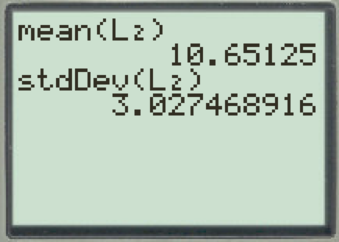
From the Ti 83 calculator output, the mean value is 10.65, and standard deviation value is 3.03.

Hence, the sample mean and the sample standard deviation by using the calculator is verified.

(b)

To determine

Find the 95% confidence interval for ${\mu }_1-{\mu }_2$.

Answer to Problem 13CRP

The 95% confidence interval for ${\mu }_1-{\mu }_2$ is $-0.06<{\mu }_1-{\mu }_2<1.60$.

Explanation of Solution

Confidence interval:

The confidence interval for ${\mu }_1-{\mu }_2$ when both ${\sigma }_1$ and ${\sigma }_2$ are unknown is,

$\left({\overline{x}}_1-{\overline{x}}_2\right)-E<{\mu }_1-{\mu }_2<\left({\overline{x}}_1-{\overline{x}}_2\right)+E$

In the formula, $s_1$ and $s_2$ are sample standard deviations of populations 1 and 2, ${\overline{x}}_1$ and ${\overline{x}}_2$ are sample means from populations 1 and 2, $n_1$ and $n_2$ are sample sizes of population 1 and 2, $E=t_c\sqrt{\frac{s_1^2}{n_1}+\frac{s_2^2}{n_2}}$, c is confidence level, and $t_c$ is the critical value for confidence level c.

The confidence level is 95%.

Critical value:

Substitute 72 for $n_1$, 80 for $n_2$ in the degrees of freedom formula.

$\begin{array}{c}d.f.=smaller\left(72-1,80-1\right)\\ =smaller\left(71,79\right)\\ =71\end{array}$

The degrees of freedom are 71.

Use the Appendix II: Tables, Table 6: Critical Values for Student’s t Distribution:

• In d.f. column locate the value 71 which is not available in the table consider as 70.
• In c row of locate the value 0.95.
• The intersecting value of row and columns is 1.994.

The critical value is 1.994.

Substitute 72 for $n_1$, 80 for $n_2$, 2.08 for $s_1$, 3.03 for $s_2$, 1.994 for $t_c$ in the margin of error formula (E).

$\begin{array}{c}E=1.994\sqrt{\frac{{2.08}^2}{72}+\frac{{3.03}^2}{80}}\\ =1.994\sqrt{0.17485}\\ =1.994\left(0.4182\right)\\ =0.83\end{array}$

The margin of error E is 0.83.

Substitute 11.42 for ${\overline{x}}_1$, 10.65 for ${\overline{x}}_2$, 0.83 for E in the confidence formula.

$\begin{array}{c}\left(11.42-10.65\right)-0.83<{\mu }_1-{\mu }_2<\left(11.42-10.65\right)+0.83\\ 0.77-0.83<{\mu }_1-{\mu }_2<0.77+0.83\\ -0.06<{\mu }_1-{\mu }_2<1.60\end{array}$

Hence, the 95% confidence interval for ${\mu }_1-{\mu }_2$ is $-0.06<{\mu }_1-{\mu }_2<1.60$.

(c)

To determine

Interpret the confidence interval in the context of the problem.

Identify whether the interval consist of numbers that are all positive or all negative or of different signs.

Explain whether mean soil water content of the first field higher than that of the second field, at 95% level of confidence.

Explanation of Solution

From part (b), the 95% confidence interval for difference between means is $-0.06<{\mu }_1-{\mu }_2<1.60$.

The confidence interval can be interpreted as; there is 95% confidence that the difference in population mean of soil water content lies within the interval –0.06 to 1.60.

It can be observed that, the 95% confidence interval calculated for difference of means $\left({\mu }_1-{\mu }_2\right)$ include both negative and positive values, that is interval contains values of different signs.

The 95% confidence interval calculated for difference of means $\left({\mu }_1-{\mu }_2\right)$ includes negative and positive values, then it cannot be determined whether ${\mu }_1-{\mu }_2>0$ or ${\mu }_1-{\mu }_2<0$. The relation between two population means cannot be either ${\mu }_1<{\mu }_2$ or ${\mu }_1>{\mu }_2$. This shows that, there would be 95% sure that there is no difference between the average of first population $\left({\mu }_1\right)$ and average of second population $\left({\mu }_2\right)$. Also, ${\mu }_1$ cannot be larger or smaller than ${\mu }_2$.

Since there is no difference between the two population means, at 95% confidence level it cannot be determined whether soil water content of the first field higher than that of the second field.

(d)

To determine

Identify and explain the distribution that is used for calculating interval.

Explain whether any additional information about the soil water content distributions is required or not.

Answer to Problem 13CRP

The distribution that is used for calculating interval is Student’s t distribution. Since the sample size is large no additional information is required.

Explanation of Solution

In the study, the population standard deviation of soil water content from field I $\left({\sigma }_1\right)$ and soil water content from field I $\left({\sigma }_2\right)$ are not known. The student’s t distribution is appropriate to used when there is no information about population standard deviation. The sample standard deviations $s_1,s_2$ are used as the estimates for ${\sigma }_1,{\sigma }_2$.

Hence, the distribution that is used for calculating interval is Student’s t distribution.

The size of first sample is $n_1=72$ and the size of second sample is $n_2=80$. It can be observed that, both the sample sizes are large $\left(n_1>30,n_2>30\right)$. This shows that, no additional information about the soil water content distribution is required since for a large sample size the sampling distribution would be normally distributed.