Videos
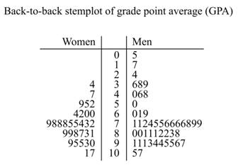
To graph: The back-to-back stem plot to represent the school performance, on the basis of grade point average (GPA) and a standardized test (IQ) of 78 seventh-grade student.
Explanation of Solution
Graph: The back-to-back stem plot is useful to compare the two related distributions by having the same stem and two leaves.
For the grade point average (GPA) of 78 seventh-grade student, draw back-to-back stemplot. The values on the left side represent the women scores and the values on the right side represent the men score. The back-to-back stemplot for comparing the distributions is shown below:
For a standardized test (IQ) of 78 seventh-grade student, draw back-to-back stemplot. The values on the left side represent the women scores and the values on the right side represent the men score. The back-to-back stemplot for comparing the distributions is shown below:
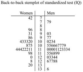
Interpretation: From the above graphs, it can be concluded that the distribution for the grade point average (GPA) and a standardized test (IQ) of 78 seventh-grade student appears almost similar.
To test: The significance difference for the grade point average (GPA) and a standardized test (IQ) of 78 seventh-grade student on the basis of gender.
Answer to Problem 137E
Solution: The difference is insignificant for the grade point average (GPA) scores of men and women. For a standardized test (IQ), the difference is insignificant as the test results are strongly significant.
Explanation of Solution
Calculation: For the difference in grade point average (GPA), the testing can be done as shown below:
The null hypothesis assumes that on an average there is no significant difference on the grade point average (GPA) scores of men and women while the alternative hypothesis assumes that on an average the grade point average (GPA) scores of men is less than the women. Symbolically, the hypothesis can be represented as follows,
Where,
To test the significant difference for the grade point averages, perform the following steps in Minitab,
Step 1: Enter the data in the worksheet of Minitab.
Step 2: Sort the data for ‘GPA’ on the basis of ‘Gender’. Here, ‘2’ represent the men and ‘1’ represent the women. Go to Data, click on sort, select ‘GPA’ in the ‘Sort column’ and enter ‘Gender’ in the ‘By column’ textbox. Also, store sorted data in the column of current worksheet. After this, make two columns, one for ‘GPA (M)’and other one for ‘GPA (F)’.
Step 3: In a Minitab worksheet go to ‘Stat’ point on ‘Basic Statistics’ and click on ‘2-Sample t’.
Step 4: In the dialogue box that appears select the samples in different column and enter the variable ‘GPA (M)’ in the first textbox and the variable ‘GPA (F)’ in the second textbox.
Step 5: Next click on options tab and set the confidence level as 95 and the Alternative hypothesis as ‘less than’. Finally click on OK twice to obtain the output.
From the Minitab results, the test statistic value is obtained as
For the difference in the standardized test (IQ) scores, the testing can be done as shown below:
The null hypothesis assumes that on an average there is no significant difference between the standardized test (IQ) scores of men and women while the alternative hypothesis assumes that on an average the standardized test (IQ) scores of men is greater than the women. Symbolically, the hypothesis can be represented as follows,
Where,
To test the significant difference for the standardized test (IQ) scores, perform the following steps in Minitab,
Step 1: Enter the data in the worksheet of Minitab.
Step 2: Sort the data for ‘IQ’ on the basis of ‘Gender’. Here, ‘2’ represent the men and ‘1’ represent the women. Go to Data, click on sort, select ‘IQ’ in the ‘Sort column’ and enter ‘Gender’ in the ‘By column’ textbox. Also, store sorted data in the column of current worksheet. After this, make two columns, one for ‘IQ (M)’and other one for ‘IQ (F)’.
Step 3: In a Minitab worksheet go to ‘Stat’ point on ‘Basic Statistics’ and click on ‘2-Sample t’.
Step 4: In the dialogue box that appears select the samples in different column and enter the variable ‘IQ (M)’ in the first textbox and the variable ‘IQ (F)’ in the second textbox.
Step 5: Next click on options tab and set the confidence level as 95 and the Alternative hypothesis as ‘greater than’. Finally click on OK twice to obtain the output.
From the Minitab results, the test statistic value is obtained as
Conclusion: Hence, for the grade point average (GPA), the P-value is greater than 0.05, so at 5% level of significance the null hypothesis will be accepted and it is concluded that the difference is insignificant. For the standardized test (IQ) scores, the P-value is greater than 0.05, so at 5% level of significance, the null hypothesis will be accepted and it is concluded that the difference is insignificant.
To find: The 95% confidence intervals for the grade point average (GPA) and the standardized test (IQ) scores of 78 seventh-grade student on the basis of gender.
Answer to Problem 137E
Solution: For the grade point average (GPA), the confidence interval is
Explanation of Solution
Calculation: The 95% confidence intervals for the grade point average (GPA) is obtained by performing the following steps in Minitab,
Step 1: Enter the data in the worksheet of Minitab.
Step 2: Sort the data for ‘GPA’ on the basis of ‘Gender’. Here, ‘2’ represent the men and ‘1’ represent the women. Go to Data, click on sort, select ‘GPA’ in the ‘Sort column’ and enter ‘Gender’ in the ‘By column’ textbox. Also, store sorted data in the column of current worksheet. After this, make two columns, one for ‘GPA (M)’and other one for ‘GPA (F)’.
Step 3: In a Minitab worksheet go to ‘Stat’ point on ‘Basic Statistics’ and click on ‘2-Sample t’.
Step 4: In the dialogue box that appears select the samples in different column and enter the variable ‘GPA (M)’ in the first textbox and the variable ‘GPA (F)’ in the second textbox.
Step 5: Next click on options tab and set the confidence level as 95 and the Alternative hypothesis as ‘not equal to’. Finally click on OK twice to obtain the output.
Hence, the confidence interval is obtained as
The 95% confidence intervals for the standardized test (IQ) scores is obtained by performing the following steps in Minitab,
Step 1: Enter the data in the worksheet of Minitab.
Step 2: Sort the data for ‘IQ’ on the basis of ‘Gender’. Here, ‘2’ represent the men and ‘1’ represent the women. Go to Data, click on sort, select ‘IQ’ in the ‘Sort column’ and enter ‘Gender’ in the ‘By column’ textbox. Also, store sorted data in the column of current worksheet. After this, make two columns, one for ‘IQ (M)’and other one for ‘IQ (F)’.
Step 3: In a Minitab worksheet go to ‘Stat’ point on ‘Basic Statistics’ and click on ‘2-Sample t’.
Step 4: In the dialogue box that appears select the samples in different column and enter the variable ‘IQ (M)’ in the first textbox and the variable ‘IQ (F)’ in the second textbox.
Step 5: Next click on options tab and set the confidence level as 95 and the Alternative hypothesis as ‘not equal to’. Finally click on OK twice to obtain the output.
Hence, the confidence interval is obtained as
Interpretation: Therefore, it can be concluded that the 95% of the average standardized IQ scores lie between the values
To explain: The findings of the graphical displays, significant test, and confidence intervals for the grade point average (GPA) and a standardized test (IQ) on the basis of gender.
Answer to Problem 137E
Solution: For the grade point average (GPA) and a standardized test (IQ), the results are not significant as the P-value in both the cases are greater than the level of significance 0.05. Also, the distribution appears to be similar in both the cases.
Explanation of Solution
For the grade point average (GPA), the test statistic is
Want to see more full solutions like this?
Chapter 7 Solutions
Introduction to the Practice of Statistics: w/CrunchIt/EESEE Access Card


- II Consider the following data matrix X: X1 X2 0.5 0.4 0.2 0.5 0.5 0.5 10.3 10 10.1 10.4 10.1 10.5 What will the resulting clusters be when using the k-Means method with k = 2. In your own words, explain why this result is indeed expected, i.e. why this clustering minimises the ESS map.arrow_forwardwhy the answer is 3 and 10?arrow_forwardPS 9 Two films are shown on screen A and screen B at a cinema each evening. The numbers of people viewing the films on 12 consecutive evenings are shown in the back-to-back stem-and-leaf diagram. Screen A (12) Screen B (12) 8 037 34 7 6 4 0 534 74 1645678 92 71689 Key: 116|4 represents 61 viewers for A and 64 viewers for B A second stem-and-leaf diagram (with rows of the same width as the previous diagram) is drawn showing the total number of people viewing films at the cinema on each of these 12 evenings. Find the least and greatest possible number of rows that this second diagram could have. TIP On the evening when 30 people viewed films on screen A, there could have been as few as 37 or as many as 79 people viewing films on screen B.arrow_forward
- Q.2.4 There are twelve (12) teams participating in a pub quiz. What is the probability of correctly predicting the top three teams at the end of the competition, in the correct order? Give your final answer as a fraction in its simplest form.arrow_forwardThe table below indicates the number of years of experience of a sample of employees who work on a particular production line and the corresponding number of units of a good that each employee produced last month. Years of Experience (x) Number of Goods (y) 11 63 5 57 1 48 4 54 5 45 3 51 Q.1.1 By completing the table below and then applying the relevant formulae, determine the line of best fit for this bivariate data set. Do NOT change the units for the variables. X y X2 xy Ex= Ey= EX2 EXY= Q.1.2 Estimate the number of units of the good that would have been produced last month by an employee with 8 years of experience. Q.1.3 Using your calculator, determine the coefficient of correlation for the data set. Interpret your answer. Q.1.4 Compute the coefficient of determination for the data set. Interpret your answer.arrow_forwardCan you answer this question for mearrow_forward
- Techniques QUAT6221 2025 PT B... TM Tabudi Maphoru Activities Assessments Class Progress lIE Library • Help v The table below shows the prices (R) and quantities (kg) of rice, meat and potatoes items bought during 2013 and 2014: 2013 2014 P1Qo PoQo Q1Po P1Q1 Price Ро Quantity Qo Price P1 Quantity Q1 Rice 7 80 6 70 480 560 490 420 Meat 30 50 35 60 1 750 1 500 1 800 2 100 Potatoes 3 100 3 100 300 300 300 300 TOTAL 40 230 44 230 2 530 2 360 2 590 2 820 Instructions: 1 Corall dawn to tha bottom of thir ceraan urina se se tha haca nariad in archerca antarand cubmit Q Search ENG US 口X 2025/05arrow_forwardThe table below indicates the number of years of experience of a sample of employees who work on a particular production line and the corresponding number of units of a good that each employee produced last month. Years of Experience (x) Number of Goods (y) 11 63 5 57 1 48 4 54 45 3 51 Q.1.1 By completing the table below and then applying the relevant formulae, determine the line of best fit for this bivariate data set. Do NOT change the units for the variables. X y X2 xy Ex= Ey= EX2 EXY= Q.1.2 Estimate the number of units of the good that would have been produced last month by an employee with 8 years of experience. Q.1.3 Using your calculator, determine the coefficient of correlation for the data set. Interpret your answer. Q.1.4 Compute the coefficient of determination for the data set. Interpret your answer.arrow_forwardQ.3.2 A sample of consumers was asked to name their favourite fruit. The results regarding the popularity of the different fruits are given in the following table. Type of Fruit Number of Consumers Banana 25 Apple 20 Orange 5 TOTAL 50 Draw a bar chart to graphically illustrate the results given in the table.arrow_forward
- Q.2.3 The probability that a randomly selected employee of Company Z is female is 0.75. The probability that an employee of the same company works in the Production department, given that the employee is female, is 0.25. What is the probability that a randomly selected employee of the company will be female and will work in the Production department? Q.2.4 There are twelve (12) teams participating in a pub quiz. What is the probability of correctly predicting the top three teams at the end of the competition, in the correct order? Give your final answer as a fraction in its simplest form.arrow_forwardQ.2.1 A bag contains 13 red and 9 green marbles. You are asked to select two (2) marbles from the bag. The first marble selected will not be placed back into the bag. Q.2.1.1 Construct a probability tree to indicate the various possible outcomes and their probabilities (as fractions). Q.2.1.2 What is the probability that the two selected marbles will be the same colour? Q.2.2 The following contingency table gives the results of a sample survey of South African male and female respondents with regard to their preferred brand of sports watch: PREFERRED BRAND OF SPORTS WATCH Samsung Apple Garmin TOTAL No. of Females 30 100 40 170 No. of Males 75 125 80 280 TOTAL 105 225 120 450 Q.2.2.1 What is the probability of randomly selecting a respondent from the sample who prefers Garmin? Q.2.2.2 What is the probability of randomly selecting a respondent from the sample who is not female? Q.2.2.3 What is the probability of randomly…arrow_forwardTest the claim that a student's pulse rate is different when taking a quiz than attending a regular class. The mean pulse rate difference is 2.7 with 10 students. Use a significance level of 0.005. Pulse rate difference(Quiz - Lecture) 2 -1 5 -8 1 20 15 -4 9 -12arrow_forward
 MATLAB: An Introduction with ApplicationsStatisticsISBN:9781119256830Author:Amos GilatPublisher:John Wiley & Sons Inc
 Probability and Statistics for Engineering and th...StatisticsISBN:9781305251809Author:Jay L. DevorePublisher:Cengage Learning
 Statistics for The Behavioral Sciences (MindTap C...StatisticsISBN:9781305504912Author:Frederick J Gravetter, Larry B. WallnauPublisher:Cengage Learning
 Elementary Statistics: Picturing the World (7th E...StatisticsISBN:9780134683416Author:Ron Larson, Betsy FarberPublisher:PEARSON
 The Basic Practice of StatisticsStatisticsISBN:9781319042578Author:David S. Moore, William I. Notz, Michael A. FlignerPublisher:W. H. Freeman
 Introduction to the Practice of StatisticsStatisticsISBN:9781319013387Author:David S. Moore, George P. McCabe, Bruce A. CraigPublisher:W. H. Freeman