Concept explainers
Videos
The modified model of the system shown in figure 1 for the gear pair attached between the motor shaft and the load. Also, compute the transfer functions
Answer to Problem 6.36P
The system’s modified model comprises the following equations as shown:
Also, the transfer functions are as follows:
Explanation of Solution
Given:
The speed control system for the field-controlled motor has been given as shown in figure 1:
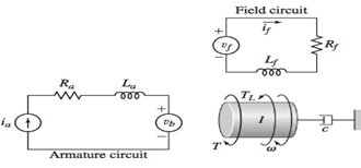
Figure 1
This speed-control system is equipped with a gear train of ratio N such that:
Concept Used:
- The system model equations for this speed-control system are as follows:
- The effective inertia and the effective damping for the rotational part equipped with a gear train of ratio N are as follows:
For field-circuit,
For rotational coupling,
Here, I and c are the effective inertia and effective damping of the system respectively.
Calculation:
The model equations for the system are:
For the inertia
Also, on considering the effect of gearbox in a rotational system, we get
Effective inertia,
Effective damping,
Thus, on using equations (2), (3) and (4), we have for effective inertia
Taking Laplace transform of equation (1) and (5) while keeping zero initial conditions, we have
From equations (6) and (7)
In case, for the multiple inputs system, for finding the transfer function for one system other inputs are temporarily set to zero that is,
For
Similarly, for
Conclusion:
The system’s modified model comprises the following equations as shown:
Also, the transfer functions are as follows:
Want to see more full solutions like this?
Chapter 6 Solutions
System Dynamics


- ### Superheated steam powers a steam turbine for the production of electrical energy. The steam expands in the turbine and at an intermediate expansion pressure (0.1 Mpa) a fraction is extracted for a regeneration process in a surface regenerator. The turbine has an isentropic efficiency of 90% Design the simplified power plant schematic Analyze it on the basis of the attached figure Determine the power generated and the thermal efficiency of the plant ### Dados in the attached imagesarrow_forwardThe machine below forms metal plates through the application of force. Two toggles (ABC and DEF) transfer forces from the central hydraulic cylinder (H) to the plates that will be formed. The toggles then push bar G to the right, which then presses a plate (p) into the cavity, thus shaping it. In this case, the plate becomes a section of a sphere. If the hydraulic cylinder can produce a maximum force of F = 10 kN, then what is the maximum P value (i.e. Pmax) that can be applied to the plate when θ = 35°? Also, what are the compressive forces in the toggle rods in that situation? Finally, what happens to Pmax and the forces in the rods as θ decreases in magnitude?arrow_forwardDetermine the magnitude of the minimum force P needed to prevent the 20 kg uniform rod AB from sliding. The contact surface at A is smooth, whereas the coefficient of static friction between the rod and the floor is μs = 0.3.arrow_forward
- Determine the magnitudes of the reactions at the fixed support at A.arrow_forwardLet Hill frame H = {i-hat_r, i-hat_θ, i-hat_h} be the orbit frame of the LMO satellite. These base vectors are generally defined as:i-hat_r = r_LM / |r_LM|, i-hat_theta = i-hat_h X i-hat_r, i-hat_h = r_LM X r-dot_LMO /( | r_LM X r-dot_LMO | ) How would you: • Determine an analytic expressions for [HN]arrow_forwardDe Moivre’s Theoremarrow_forward
- hand-written solutions only, please.arrow_forwardDetermine the shear flow qqq for the given profile when the shear forces acting at the torsional center are Qy=30Q_y = 30Qy=30 kN and Qz=20Q_z = 20Qz=20 kN. Also, calculate qmaxq_{\max}qmax and τmax\tau_{\max}τmax. Given:Iy=10.5×10⁶I_y = 10.5 \times 10^6Iy=10.5×106 mm4^44,Iz=20.8×10⁶I_z = 20.8 \times 10^6Iz=20.8×106 mm4^44,Iyz=6×10⁶I_{yz} = 6 \times 10^6Iyz=6×106 mm4^44. Additional parameters:αy=0.5714\alpha_y = 0.5714αy=0.5714,αz=0.2885\alpha_z = 0.2885αz=0.2885,γ=1.1974\gamma = 1.1974γ=1.1974. (Check hint: τmax\tau_{\max}τmax should be approximately 30 MPa.)arrow_forwardhand-written solutions only, please.arrow_forward
- In the bending of a U-profile beam, the load path passes through the torsional center C, causing a moment of 25 kNm at the cross-section under consideration. Additionally, the beam is subjected to an axial tensile force of 100 kN at the centroid. Determine the maximum absolute normal stress.(Check hint: approximately 350 MPa, but where?)arrow_forward### Make an introduction to a report of a rocket study project, in the OpenRocket software, where the project consists of the simulation of single-stage and two-stage rockets, estimating the values of the exhaust velocities of the engines used, as well as obtaining the graphs of "altitude", "mass ratio x t", "thrust x t" and "ψ × t".arrow_forwardA 6305 ball bearing is subjected to a steady 5000-N radial load and a 2000-N thrust load and uses a very clean lubricant throughout its life. If the inner race angular velocity is 500 rpm find The equivalent radial load the L10 life and the L50 lifearrow_forward
 Elements Of ElectromagneticsMechanical EngineeringISBN:9780190698614Author:Sadiku, Matthew N. O.Publisher:Oxford University Press
 Mechanics of Materials (10th Edition)Mechanical EngineeringISBN:9780134319650Author:Russell C. HibbelerPublisher:PEARSON
 Thermodynamics: An Engineering ApproachMechanical EngineeringISBN:9781259822674Author:Yunus A. Cengel Dr., Michael A. BolesPublisher:McGraw-Hill Education
 Control Systems EngineeringMechanical EngineeringISBN:9781118170519Author:Norman S. NisePublisher:WILEY
 Mechanics of Materials (MindTap Course List)Mechanical EngineeringISBN:9781337093347Author:Barry J. Goodno, James M. GerePublisher:Cengage Learning
 Engineering Mechanics: StaticsMechanical EngineeringISBN:9781118807330Author:James L. Meriam, L. G. Kraige, J. N. BoltonPublisher:WILEY