Videos
Determine the roots of the simultaneous nonlinear equations
Use a graphical approach to obtain your initial guesses. Determine refined estimates with the two-equation Newton-Raphson method described in Sec. 6.6.2.
To calculate: The root of the non-linear simultaneous equations,
By the two-equation Newton-Raphson method and find the initial guess by the graphical method.
Answer to Problem 23P
Solution:
The root of the simultaneous non-linear equations
For the initial root
For the initial root
Explanation of Solution
Given information:
The non-linear simultaneous equation,
Formula used:
The Newton-Raphson formula for two non-linear equation is,
Calculation:
Use MATLAB to draw the graph of the equations,
Code:
%x-coordinates spacing is defined.
%first function is defined.
%second function is defined.
%Plot command is used to draw the two function.
Output:
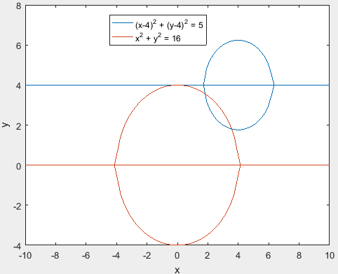
From the above graph, it is observed that there are two roots at
Consider theequations,
Rewrite the equation as below,
Partial differentiate the above functions with respect to x,
And,
Now, partial differentiate the above functions with respect to y,
And,
Use initial guesses
And,
Now, use
And,
Now, use
And,
Thus, all the iteration can be summarized as below,
| 0 | 1.8 | 3.6 |
| 1 | 1.8056 | 3.5694 |
| 2 | 1.80583 | 3.56917 |
| 3 | 1.80583 | 3.56917 |
Hence, the root of the simultaneous non-linear equations
Use initial guesses
And,
Now, use
And,
Now, use
And,
Thus, all the iteration can be summarized as below,
| 0 | 3.6 | 1.8 |
| 1 | 3.56944 | 1.80556 |
| 2 | 3.56917 | 1.80583 |
| 3 | 3.56917 | 1.80583 |
Hence, the root of the simultaneous non-linear equations
Want to see more full solutions like this?
Chapter 6 Solutions
EBK NUMERICAL METHODS FOR ENGINEERS
Additional Engineering Textbook Solutions
College Algebra (Collegiate Math)
Pathways To Math Literacy (looseleaf)
Graphical Approach To College Algebra
Probability And Statistical Inference (10th Edition)
Elementary Statistics: Picturing the World (7th Edition)


- For each month of the year, Taylor collected the average high temperatures in Jackson, Mississippi. He used the data to create the histogram shown. Which set of data did he use to create the histogram? A 55, 60, 64, 72, 73, 75, 77, 81, 83, 91, 91, 92\ 55,\ 60,\ 64,\ 72,\ 73,\ 75,\ 77,\ 81,\ 83,\ 91,\ 91,\ 92 55, 60, 64, 72, 73, 75, 77, 81, 83, 91, 91, 92 B 55, 57, 60, 65, 70, 71, 78, 79, 85, 86, 88, 91\ 55,\ 57,\ 60,\ 65,\ 70,\ 71,\ 78,\ 79,\ 85,\ 86,\ 88,\ 91 55, 57, 60, 65, 70, 71, 78, 79, 85, 86, 88, 91 C 55, 60, 63, 64, 65, 71, 83, 87, 88, 88, 89, 93\ 55,\ 60,\ 63,\ 64,\ 65,\ 71,\ 83,\ 87,\ 88,\ 88,\ 89,\ 93 55, 60, 63, 64, 65, 71, 83, 87, 88, 88, 89, 93 D 55, 58, 60, 66, 68, 75, 77, 82, 86, 89, 91, 91\ 55,\ 58,\ 60,\ 66,\ 68,\ 75,\ 77,\ 82,\ 86,\ 89,\ 91,\ 91 55, 58, 60, 66, 68, 75, 77, 82, 86, 89, 91, 91arrow_forward3. Consider the polynomial equation 6-iz+7z2-iz³ +z = 0 for which the roots are 3i, -2i, -i, and i. (a) Verify the relations between this roots and the coefficients of the polynomial. (b) Find the annulus region in which the roots lie.arrow_forwardc) Using only Laplace transforms solve the following Samuelson model given below i.e., the second order difference equation (where yt is national income): - Yt+2 6yt+1+5y₁ = 0, if y₁ = 0 for t < 0, and y₁ = 0, y₁ = 1 1-e-s You may use without proof that L-1[s(1-re-s)] = f(t) = r² for n ≤tarrow_forwardScoring: MATH 15 FILING /10 COMPARISON /10 RULER I 13 Express EMPLOYMENT PROFESSIONALS NAME: SKILLS EVALUATION TEST- Light Industrial MATH-Solve the following problems. (Feel free to use a calculator.) DATE: 1. If you were asked to load 225 boxes onto a truck, and the boxes are crated, with each crate containing nine boxes, how many crates would you need to load? 2. Imagine you live only one mile from work and you decide to walk. If you walk four miles per hour, how long will it take you to walk one mile? 3. Add 3 feet 6 inches + 8 feet 2 inches + 4 inches + 2 feet 5 inches. 4. In a grocery store, steak costs $3.85 per pound. If you buy a three-pound steak and pay for it with a $20 bill, how much change will you get? 5. Add 8 minutes 32 seconds + 37 minutes 18 seconds + 15 seconds. FILING - In the space provided, write the number of the file cabinet where the company should be filed. Example: File Cabinet #4 Elson Co. File Cabinets: 1. Aa-Bb 3. Cg-Dz 5. Ga-Hz 7. La-Md 9. Na-Oz 2. Bc-Cf…arrow_forwardIf you were asked to load 225 boxes onto a truck, and the boxes are crated, with each crate containing nine boxes, how many crates would you need to load?arrow_forwardHabitat for Humanity International is a nonprofit organization dedicated to eliminating poverty housing worldwide. Suppose the following table contains estimates of activity times (in days) involved in the construction of a house that Habitat for Humanity is building. Activity Optimistic Most Probable Pessimistic A 6 7.0 8 B 7 8.0 9 C 7 7.5 11.5 D 7 9.0 10 E 6 7.0 9 F 3 4.0 5 (a) Compute the expected activity completion times and the variance for each activity. (Round your answers to two decimal places.) Activity Expected Times A B C D E F Variance (b) An analyst determined that the critical path consists of activities B-D-F. Compute the expected project completion time and the variance of this path. (Round your answers to two decimal places.) expected project completion time variance of projection completion timearrow_forwardTo manage the production of an animated movie, Pixar Animation Studios has listed the major activities involved, the predecessor relationships, and activity times (in months). The project is completed when activities F and G are both complete. Activity Immediate Predecessor G A B CD E A A C, B C, B D, E Time 4 6 2 6 3 3 5 (a) Find the critical path. (Enter your answers as a comma-separated list.) (b) The project must be completed in 1.5 years. Do you anticipate difficulty in meeting the deadline? Explain. The critical path activities require months to complete. Thus the project ---Select--- be completed in 1.5 years.arrow_forwardTo help with preparations, a couple has devised a project network to describe the activities that must be completed by their wedding date. In addition, they have estimated the time of each activity (in weeks). Start D F B E G Activity A B C DEFGH Time 5 3 6 6 6 3 11 10 (a) Identify the critical path. (Enter your answers as a comma-separated list.) H Finish (b) How much time (in weeks) will be needed to complete this project? week(s) (c) Can activity D be delayed without delaying the entire project? If so, by how many weeks? (If the activity can not be delayed, enter 0.) week(s) (d) Can activity C be delayed without delaying the entire project? If so, by how many weeks? (If the activity can not be delayed, enter 0.) week(s) (e) What is the schedule for activity E (in weeks)? Earliest Start Latest Start Earliest Finish Latest Finish week(s) week(s) week(s) week(s)arrow_forward30.6. Classify the zeros and singularities of the functions tanz (a). f(z)=sin(1-2-1), (b). f(2) = (c). f(z)= tanh .arrow_forward1. Locate the singularities of three of the following functions, and determine their type. (a) f(z)=2(z-sinz). (b) f(z) = (-) (c) f(z) = (z+2-22²)-1 (d) f(z) = sinzarrow_forwardQ 2/classify the zeros and poles of the function f(z) = tanz Zarrow_forward30.1. Show that z = 0 is a removable singularity of the following functions. Furthermore, define f(0) such that these functions are analytic at z = 0. (a). f(z) = 2 sin z- z 1-12² - cos z (b). f(z) = (c). f(z) = sin 22arrow_forwardarrow_back_iosSEE MORE QUESTIONSarrow_forward_ios
 Algebra & Trigonometry with Analytic GeometryAlgebraISBN:9781133382119Author:SwokowskiPublisher:Cengage