
Concept explainers
Videos
To determine: In this problem, by using the ticker symbol given, the five year data of monthly adjusted stock prices can be downloaded. After that returns can be calculated and returns data of respective company can be plotted on xy scatter plot against the data of S&P. Then by following the steps mentioned in the questions trend line can be made. Slope of the trend line will be beta of the stock.
Explanation of Solution
First we have to down load the data of Eli Lilly (LLY) for the period between Jan 2014 and Nov 2018 (Five years). Then the returns can be calculated by using this formula:
Where LN is natural logarithm
Now this is the calculated data here under for Eli Lily. Similarly S&P Data can be obtained and Returns can be calculated as mentioned above.
| LLY Company | S&P 500 | ||||
| Date | Adj Close | Return LLY | Date | Adj Close | Return S&P |
| 12/1/2013 | null | 0 | 12/1/2013 | null | 0 |
| 1/1/2014 | 46.83643 | 0 | 1/1/2014 | 1782.59 | 0 |
| 2/1/2014 | 51.692627 | 0.0986538 | 2/1/2014 | 1859.45 | 0.04221337 |
| 3/1/2014 | 51.505238 | -0.003632 | 3/1/2014 | 1872.34 | 0.00690825 |
| 4/1/2014 | 51.715252 | 0.0040692 | 4/1/2014 | 1883.95 | 0.00618164 |
| 5/1/2014 | 52.380283 | 0.0127775 | 5/1/2014 | 1923.57 | 0.0208122 |
| 6/1/2014 | 54.853989 | 0.0461447 | 6/1/2014 | 1960.23 | 0.018879 |
| 7/1/2014 | 53.874619 | -0.018015 | 7/1/2014 | 1930.67 | -0.0151947 |
| 8/1/2014 | 56.08041 | 0.0401271 | 8/1/2014 | 2003.37 | 0.03696364 |
| 9/1/2014 | 57.679146 | 0.0281091 | 9/1/2014 | 1972.29 | -0.0156354 |
| 10/1/2014 | 58.995499 | 0.0225655 | 10/1/2014 | 2018.05 | 0.0229364 |
| 11/1/2014 | 60.587559 | 0.0266284 | 11/1/2014 | 2067.56 | 0.02423747 |
| 12/1/2014 | 61.807735 | 0.0199389 | 12/1/2014 | 2058.9 | -0.0041974 |
| 1/1/2015 | 64.504379 | 0.0427046 | 1/1/2015 | 1994.99 | -0.0315328 |
| 2/1/2015 | 62.864899 | -0.025745 | 2/1/2015 | 2104.5 | 0.05343888 |
| 3/1/2015 | 65.551598 | 0.0418496 | 3/1/2015 | 2067.89 | -0.0175492 |
| 4/1/2015 | 64.847809 | -0.010794 | 4/1/2015 | 2085.51 | 0.00848472 |
| 5/1/2015 | 71.190941 | 0.0933225 | 5/1/2015 | 2107.39 | 0.01043673 |
| 6/1/2015 | 75.853432 | 0.0634374 | 6/1/2015 | 2063.11 | -0.0212356 |
| 7/1/2015 | 76.780136 | 0.012143 | 7/1/2015 | 2103.84 | 0.01954968 |
| 8/1/2015 | 74.817703 | -0.025891 | 8/1/2015 | 1972.18 | -0.0646247 |
| 9/1/2015 | 76.492958 | 0.0221442 | 9/1/2015 | 1920.03 | -0.0267987 |
| 10/1/2015 | 74.555267 | -0.025658 | 10/1/2015 | 2079.36 | 0.07971938 |
| 11/1/2015 | 74.984871 | 0.0057457 | 11/1/2015 | 2080.41 | 0.00050474 |
| 12/1/2015 | 77.502235 | 0.0330204 | 12/1/2015 | 2043.94 | -0.0176857 |
| 1/1/2016 | 72.756081 | -0.063194 | 1/1/2016 | 1940.24 | -0.0520676 |
| 2/1/2016 | 66.22551 | -0.094047 | 2/1/2016 | 1932.23 | -0.0041369 |
| 3/1/2016 | 66.695992 | 0.0070791 | 3/1/2016 | 2059.74 | 0.06390499 |
| 4/1/2016 | 69.95623 | 0.0477249 | 4/1/2016 | 2065.3 | 0.00269576 |
| 5/1/2016 | 69.493126 | -0.006642 | 5/1/2016 | 2096.95 | 0.01520837 |
| 6/1/2016 | 73.425682 | 0.0550459 | 6/1/2016 | 2098.86 | 0.00091051 |
| 7/1/2016 | 77.285789 | 0.0512363 | 7/1/2016 | 2173.6 | 0.03499043 |
| 8/1/2016 | 72.493301 | -0.064016 | 8/1/2016 | 2170.95 | -0.00122 |
| 9/1/2016 | 75.310425 | 0.0381244 | 9/1/2016 | 2168.27 | -0.0012352 |
| 10/1/2016 | 69.286331 | -0.083371 | 10/1/2016 | 2126.15 | -0.0196168 |
| 11/1/2016 | 62.980747 | -0.095419 | 11/1/2016 | 2198.81 | 0.03360355 |
| 12/1/2016 | 69.921356 | 0.104542 | 12/1/2016 | 2238.83 | 0.01803711 |
| 1/1/2017 | 73.229668 | 0.0462295 | 1/1/2017 | 2278.87 | 0.01772631 |
| 2/1/2017 | 78.724503 | 0.0723538 | 2/1/2017 | 2363.64 | 0.036523 |
| 3/1/2017 | 80.498466 | 0.0222837 | 3/1/2017 | 2362.72 | -0.0003893 |
| 4/1/2017 | 78.536491 | -0.024675 | 4/1/2017 | 2384.2 | 0.00905013 |
| 5/1/2017 | 76.153404 | -0.030814 | 5/1/2017 | 2411.8 | 0.01150976 |
| 6/1/2017 | 79.274796 | 0.0401705 | 6/1/2017 | 2423.41 | 0.00480223 |
| 7/1/2017 | 79.621574 | 0.0043648 | 7/1/2017 | 2470.3 | 0.01916402 |
| 8/1/2017 | 78.301926 | -0.016713 | 8/1/2017 | 2471.65 | 0.00054628 |
| 9/1/2017 | 82.921219 | 0.0573188 | 9/1/2017 | 2519.36 | 0.01911904 |
| 10/1/2017 | 79.431435 | -0.042997 | 10/1/2017 | 2575.26 | 0.02194556 |
| 11/1/2017 | 82.048775 | 0.0324197 | 11/1/2017 | 2584.84 | 0.00371314 |
| 12/1/2017 | 82.39135 | 0.0041666 | 12/1/2017 | 2673.61 | 0.03376601 |
| 1/1/2018 | 79.45507 | -0.036289 | 1/1/2018 | 2823.81 | 0.0546574 |
| 2/1/2018 | 75.133568 | -0.055924 | 2/1/2018 | 2713.83 | -0.0397261 |
| 3/1/2018 | 76.036209 | 0.0119422 | 3/1/2018 | 2640.87 | -0.0272525 |
| 4/1/2018 | 79.672424 | 0.0467139 | 4/1/2018 | 2648.05 | 0.00271509 |
| 5/1/2018 | 83.573997 | 0.0478089 | 5/1/2018 | 2705.27 | 0.02137819 |
| 6/1/2018 | 84.436729 | 0.0102701 | 6/1/2018 | 2718.37 | 0.00483075 |
| 7/1/2018 | 97.77562 | 0.1466728 | 7/1/2018 | 2816.29 | 0.03538795 |
| 8/1/2018 | 104.544014 | 0.0669329 | 8/1/2018 | 2901.52 | 0.02981431 |
| 9/1/2018 | 106.772926 | 0.0210962 | 9/1/2018 | 2913.98 | 0.00428509 |
| 10/1/2018 | 107.89727 | 0.0104752 | 10/1/2018 | 2711.74 | -0.0719293 |
| 11/1/2018 | 118.046219 | 0.0898967 | 11/1/2018 | 2760.17 | 0.01770175 |
| 12/1/2018 | 115.839996 | -0.018866 | 12/1/2018 | 2695.95 | -0.0235416 |
| 12/6/2018 | 115.839996 | 0 | 12/6/2018 | 2695.95 | 0 |
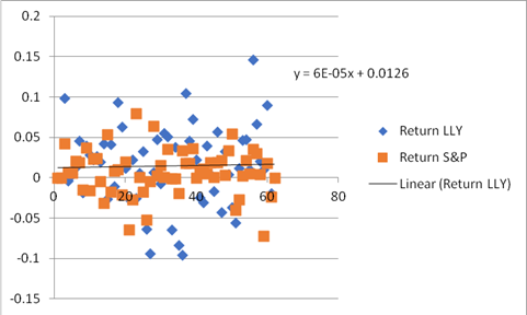
Now scatter plot between return of Eli Lilly and S&P 500 can be made like this:
The trend line can also be obtained by clicking on any blue point and following the steps. This trend line shows that the slope is -0.0004. This slope is beta of Stock Eli Lilly.
Similarly data can be obtained for the next firm AA and returns can be calculated.
| AA Company | S&P 500 | ||||
| Date | Adj Close | Return AA | Date | Adj Close | Return S&P |
| 12/1/2013 | null | 0 | 12/1/2013 | null | 0 |
| 1/1/2014 | 26.76451 | 0 | 1/1/2014 | 1782.59 | 0 |
| 2/1/2014 | 27.29933 | 0.019786 | 2/1/2014 | 1859.45 | 0.04221337 |
| 3/1/2014 | 30.00557 | 0.094521 | 3/1/2014 | 1872.34 | 0.00690825 |
| 4/1/2014 | 31.40442 | 0.045566 | 4/1/2014 | 1883.95 | 0.00618164 |
| 5/1/2014 | 31.73083 | 0.01034 | 5/1/2014 | 1923.57 | 0.0208122 |
| 6/1/2014 | 34.79342 | 0.09214 | 6/1/2014 | 1960.23 | 0.018879 |
| 7/1/2014 | 38.29848 | 0.095982 | 7/1/2014 | 1930.67 | -0.0151947 |
| 8/1/2014 | 38.81255 | 0.013333 | 8/1/2014 | 2003.37 | 0.03696364 |
| 9/1/2014 | 37.6662 | -0.02998 | 9/1/2014 | 1972.29 | -0.0156354 |
| 10/1/2014 | 39.23465 | 0.040797 | 10/1/2014 | 2018.05 | 0.0229364 |
| 11/1/2014 | 40.47537 | 0.031133 | 11/1/2014 | 2067.56 | 0.02423747 |
| 12/1/2014 | 37.031 | -0.08894 | 12/1/2014 | 2058.9 | -0.0041974 |
| 1/1/2015 | 36.70266 | -0.00891 | 1/1/2015 | 1994.99 | -0.0315328 |
| 2/1/2015 | 34.68578 | -0.05652 | 2/1/2015 | 2104.5 | 0.05343888 |
| 3/1/2015 | 30.35504 | -0.13337 | 3/1/2015 | 2067.89 | -0.0175492 |
| 4/1/2015 | 31.52978 | 0.03797 | 4/1/2015 | 2085.51 | 0.00848472 |
| 5/1/2015 | 29.36827 | -0.07102 | 5/1/2015 | 2107.39 | 0.01043673 |
| 6/1/2015 | 26.25399 | -0.1121 | 6/1/2015 | 2063.11 | -0.0212356 |
| 7/1/2015 | 23.24008 | -0.12194 | 7/1/2015 | 2103.84 | 0.01954968 |
| 8/1/2015 | 22.25113 | -0.04349 | 8/1/2015 | 1972.18 | -0.0646247 |
| 9/1/2015 | 22.81595 | 0.025067 | 9/1/2015 | 1920.03 | -0.0267987 |
| 10/1/2015 | 21.09177 | -0.07858 | 10/1/2015 | 2079.36 | 0.07971938 |
| 11/1/2015 | 22.10739 | 0.047029 | 11/1/2015 | 2080.41 | 0.00050474 |
| 12/1/2015 | 23.38675 | 0.056258 | 12/1/2015 | 2043.94 | -0.0176857 |
| 1/1/2016 | 17.2735 | -0.303 | 1/1/2016 | 1940.24 | -0.0520676 |
| 2/1/2016 | 21.15944 | 0.202913 | 2/1/2016 | 1932.23 | -0.0041369 |
| 3/1/2016 | 22.79773 | 0.074575 | 3/1/2016 | 2059.74 | 0.06390499 |
| 4/1/2016 | 26.58148 | 0.153554 | 4/1/2016 | 2065.3 | 0.00269576 |
| 5/1/2016 | 22.06001 | -0.18645 | 5/1/2016 | 2096.95 | 0.01520837 |
| 6/1/2016 | 22.12414 | 0.002903 | 6/1/2016 | 2098.86 | 0.00091051 |
| 7/1/2016 | 25.3461 | 0.135956 | 7/1/2016 | 2173.6 | 0.03499043 |
| 8/1/2016 | 24.05732 | -0.05219 | 8/1/2016 | 2170.95 | -0.00122 |
| 9/1/2016 | 24.27107 | 0.008846 | 9/1/2016 | 2168.27 | -0.0012352 |
| 10/1/2016 | 21.3561 | -0.12795 | 10/1/2016 | 2126.15 | -0.0196168 |
| 11/1/2016 | 28.85664 | 0.301002 | 11/1/2016 | 2198.81 | 0.03360355 |
| 12/1/2016 | 28.08 | -0.02728 | 12/1/2016 | 2238.83 | 0.01803711 |
| 1/1/2017 | 36.45 | 0.260884 | 1/1/2017 | 2278.87 | 0.01772631 |
| 2/1/2017 | 34.59 | -0.05238 | 2/1/2017 | 2363.64 | 0.036523 |
| 3/1/2017 | 34.4 | -0.00551 | 3/1/2017 | 2362.72 | -0.0003893 |
| 4/1/2017 | 33.73 | -0.01967 | 4/1/2017 | 2384.2 | 0.00905013 |
| 5/1/2017 | 32.94 | -0.0237 | 5/1/2017 | 2411.8 | 0.01150976 |
| 6/1/2017 | 32.65 | -0.00884 | 6/1/2017 | 2423.41 | 0.00480223 |
| 7/1/2017 | 36.4 | 0.108724 | 7/1/2017 | 2470.3 | 0.01916402 |
| 8/1/2017 | 43.88 | 0.18689 | 8/1/2017 | 2471.65 | 0.00054628 |
| 9/1/2017 | 46.62 | 0.060571 | 9/1/2017 | 2519.36 | 0.01911904 |
| 10/1/2017 | 47.78 | 0.024578 | 10/1/2017 | 2575.26 | 0.02194556 |
| 11/1/2017 | 41.51 | -0.14067 | 11/1/2017 | 2584.84 | 0.00371314 |
| 12/1/2017 | 53.87 | 0.260639 | 12/1/2017 | 2673.61 | 0.03376601 |
| 1/1/2018 | 52.02 | -0.03495 | 1/1/2018 | 2823.81 | 0.0546574 |
| 2/1/2018 | 44.97 | -0.14563 | 2/1/2018 | 2713.83 | -0.0397261 |
| 3/1/2018 | 44.96 | -0.00022 | 3/1/2018 | 2640.87 | -0.0272525 |
| 4/1/2018 | 51.2 | 0.129966 | 4/1/2018 | 2648.05 | 0.00271509 |
| 5/1/2018 | 48.07 | -0.06308 | 5/1/2018 | 2705.27 | 0.02137819 |
| 6/1/2018 | 46.88 | -0.02507 | 6/1/2018 | 2718.37 | 0.00483075 |
| 7/1/2018 | 43.27 | -0.08013 | 7/1/2018 | 2816.29 | 0.03538795 |
| 8/1/2018 | 44.67 | 0.031843 | 8/1/2018 | 2901.52 | 0.02981431 |
| 9/1/2018 | 40.4 | -0.10047 | 9/1/2018 | 2913.98 | 0.00428509 |
| 10/1/2018 | 34.99 | -0.14377 | 10/1/2018 | 2711.74 | -0.0719293 |
| 11/1/2018 | 31.81 | -0.09528 | 11/1/2018 | 2760.17 | 0.01770175 |
| 12/1/2018 | 29.65 | -0.07032 | 12/1/2018 | 2695.95 | -0.0235416 |
| 12/6/2018 | 29.65 | 0 | 12/6/2018 | 2695.95 | 0 |
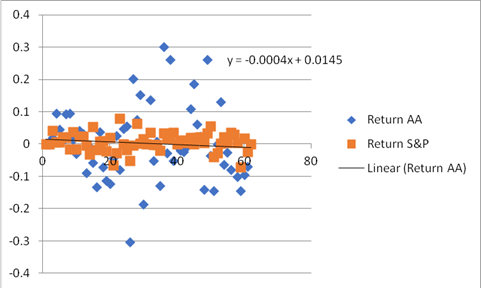
Then we can again prepare scatter plot between returns of AA and S&P like mentioned below.
Scatter Plot can be made by using MS Excel plot function by selecting Returns of LLY and S&P.4
The scatter plot will look like this.
Also then we can insert regression equation. The regression equation will look like this:
Y = 6E-05x + 0.0126
 t
t
Now from the trend line we have the slope of trend line that shows that beta of stock AA is -0.00006.
The result shows that Eli Lilly has a negative beta and AA has positive beta. Eli Lilly's negative beta is useful to diversify the portfolio in which this stock would be added, for the reason that this stock's returns are negatively correlated with market returns and thus increasing diversification, lowering risk at the cost of less expected returns.
Want to see more full solutions like this?
Chapter 6 Solutions
ESSEN.OF.INVESTMENTS+CONNECT


- An accounts payable period decrease would increase the length of a firm's cash cycle. Consider each in isolation. Question 6 options: True Falsearrow_forwardWhich of the following is the best definition of cash budget? Question 10 options: Costs that rise with increases in the level of investment in current assets. A forecast of cash receipts and disbursements for the next planning period. A secured short-term loan that involves either the assignment or factoring of the receivable. The time between sale of inventory and collection of the receivable. The time between receipt of inventory and payment for it.arrow_forwardShort-term financial decisions are typically defined to include cash inflows and outflows that occur within __ year(s) or less. Question 9 options: Four Two Three Five Onearrow_forward
- A national firm has sales of $575,000 and cost of goods sold of $368,000. At the beginning of the year, the inventory was $42,000. At the end of the year, the inventory balance was $45,000. What is the inventory turnover rate? Question 8 options: 8.46 times 13.22 times 43.14 times 12.78 times 28.56 timesarrow_forwardThe formula (Cash cycle + accounts payable period) correctly defines the operating cycle. Question 7 options: False Truearrow_forwardAn accounts payable period decrease would increase the length of a firm's cash cycle. Consider each in isolation. Question 6 options: True Falsearrow_forward
- Which of the following issues is/are NOT considered a part of short-term finance? Question 5 options: The amount of credit that should be extended to customers The firm determining whether to issue commercial paper or obtain a bank loan The amount of the firms current income that should be paid out as dividends The amount the firm should borrow short-term A reasonable level of cash for the firm to maintainarrow_forwardLiberal credit terms for customers is associated with a restrictive short-term financial policy. Question 3 options: True Falsearrow_forwardAn increase in fixed assets is a source of cash. Question 2 options: True Falsearrow_forward
- If the initial current ratio for a firm is greater than one, then using cash to purchase marketable securities will decrease net working capital. True or falsearrow_forwardwhat is going to be the value of American put option that expires in one year modeled with a binomial tree of 3 months step with year to expiry? assume the underlying is oil future with RF of 5% and vol of oil is 30%. Strike is 70 and price is 60 of oil. 13.68 13.44 13.01arrow_forwardhello tutor need step by step approach.arrow_forward
 Essentials Of InvestmentsFinanceISBN:9781260013924Author:Bodie, Zvi, Kane, Alex, MARCUS, Alan J.Publisher:Mcgraw-hill Education,

 Foundations Of FinanceFinanceISBN:9780134897264Author:KEOWN, Arthur J., Martin, John D., PETTY, J. WilliamPublisher:Pearson,
 Fundamentals of Financial Management (MindTap Cou...FinanceISBN:9781337395250Author:Eugene F. Brigham, Joel F. HoustonPublisher:Cengage Learning
 Corporate Finance (The Mcgraw-hill/Irwin Series i...FinanceISBN:9780077861759Author:Stephen A. Ross Franco Modigliani Professor of Financial Economics Professor, Randolph W Westerfield Robert R. Dockson Deans Chair in Bus. Admin., Jeffrey Jaffe, Bradford D Jordan ProfessorPublisher:McGraw-Hill Education