Concept explainers
Videos
Suppose you wish to fit a function of the form
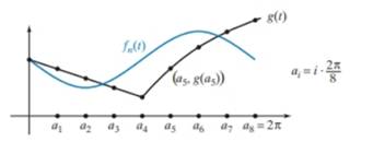
To find
or
or
where
a. Find the entries of the matrix
b. Find
Hint: Interpret the entries of the matrix
c. Find
The resulting vector
Write
Want to see the full answer?
Check out a sample textbook solution
Chapter 5 Solutions
Linear Algebra with Applications (2-Download)


- There are 25 different varieties of flowering plants found in a natural habitat you are studying. You are asked to randomly select 5 of these flowering plant varieties to bring back to your laboratory for further study. How many different combinations of are possible? That is, how many possible 5 plant subgroups can be formed out of the 25 total plants found?arrow_forwardA person is tossing a fair, two-sided coin three times and recording the results (either a Heads, H, or a Tails, T). Let E be the event that exactly two heads are tossed. Which of the following sets represent the event E? Group of answer choices {HHT, HTH, THH} {HHT, THH} {HHH, HHT, HTH, THH, TTT, TTH, THT, HTT} {HH}arrow_forwardTake Quiz 54m Exit Let the universal set be whole numbers 1 through 20 inclusive. That is, U = {1, 2, 3, 4, . . ., 19, 20}. Let A, B, and C be subsets of U. Let A be the set of all prime numbers: A = {2, 3, 5, 7, 11, 13, 17, 19} Let B be the set of all odd numbers: B = {1,3,5,7, • • , 17, 19} Let C be the set of all square numbers: C = {1,4,9,16} ☐ Question 2 3 pts Which of the following statement(s) is true? Select all that apply. (1) АСВ (2) A and C are disjoint (mutually exclusive) sets. (3) |B| = n(B) = 10 (4) All of the elements in AC are even numbers. ☐ Statement 1 is true. Statement 2 is true. Statement 3 is true. Statement 4 is true.arrow_forward
- ☐ Question 1 2 pts Let G be the set that represents all whole numbers between 5 and 12 exclusive. Which of the following is set G in standard set notation. (Roster Method)? O G = [5, 12] G = {5, 6, 7, 8, 9, 10, 11, 12} O G = (5, 12) OG = {6, 7, 8, 9, 10, 11}arrow_forwardSolve thisarrow_forwardint/PlayerHomework.aspx?homeworkId=689099898&questionId=1&flushed=false&cid=8120746¢erw BP Physical Geograph... HW Score: 0%, 0 of 13 points ○ Points: 0 of 1 Determine if the values of the variables listed are solutions of the system of equations. 2x - y = 4 3x+5y= - 6 x=1, y = 2; (1,-2) Is (1, 2) a solution of the system of equations? L No Yes iew an example Get more help - Aarrow_forward
- 12:01 PM Tue May 13 < AA ✓ Educatic S s3.amazona... A Assess Your... 目 accelerate-iu15-bssd.vschool.com S s3.amazona... Trigonometric Identities Module Exam Dashboard ... Dashboard ... Algebra 2 Pa... Algebra 2 Part 4 [Honors] (Acc. Ed.) (Zimmerman) 24-25 / Module 11: Trigonometric Identities i + 38% ✰ Start Page Alexis Forsythe All changes saved 10. A sound wave's amplitude can be modeled by the function y = −7 sin ((x-1) + 4). Within the interval 0 < x < 12, when does the function have an amplitude of 4? (Select all that apply.) 9.522 seconds 4.199 seconds 0.522 seconds 1.199 seconds Previous 10 of 20 Nextarrow_forwardJamal wants to save $48,000 for a down payment on a home. How much will he need to invest in an account with 11.8% APR, compounding daily, in order to reach his goal in 10 years? Round to the nearest dollar.arrow_forwardr nt Use the compound interest formula, A (t) = P(1 + 1)". An account is opened with an intial deposit of $7,500 and earns 3.8% interest compounded semi- annually. Round all answers to the nearest dollar. a. What will the account be worth in 10 years? $ b. What if the interest were compounding monthly? $ c. What if the interest were compounded daily (assume 365 days in a year)? $arrow_forward
- Kyoko has $10,000 that she wants to invest. Her bank has several accounts to choose from. Her goal is to have $15,000 by the time she finishes graduate school in 7 years. To the nearest hundredth of a percent, what should her minimum annual interest rate be in order to reach her goal assuming they compound daily? (Hint: solve the compound interest formula for the intrerest rate. Also, assume there are 365 days in a year) %arrow_forward3:56 wust.instructure.com Page 0 Chapter 5 Test Form A of 2 - ZOOM + | Find any real numbers for which each expression is undefined. 2x 4 1. x Name: Date: 1. 3.x-5 2. 2. x²+x-12 4x-24 3. Evaluate when x=-3. 3. x Simplify each rational expression. x²-3x 4. 2x-6 5. x²+3x-18 x²-9 6. Write an equivalent rational expression with the given denominator. 2x-3 x²+2x+1(x+1)(x+2) Perform the indicated operation and simplify if possible. x²-16 x-3 7. 3x-9 x²+2x-8 x²+9x+20 5x+25 8. 4.x 2x² 9. x-5 x-5 3 5 10. 4x-3 8x-6 2 3 11. x-4 x+4 x 12. x-2x-8 x²-4 ← -> Copyright ©2020 Pearson Education, Inc. + 5 4. 5. 6. 7. 8. 9. 10. 11. 12. T-97arrow_forwardProblem #5 Suppose you flip a two sided fair coin ("heads" or "tails") 8 total times. a). How many ways result in 6 tails and 2 heads? b). How many ways result in 2 tails and 6 heads? c). Compare your answers to part (a) and (b) and explain in a few sentences why the comparison makes sense.arrow_forward
 Algebra and Trigonometry (6th Edition)AlgebraISBN:9780134463216Author:Robert F. BlitzerPublisher:PEARSON
 Contemporary Abstract AlgebraAlgebraISBN:9781305657960Author:Joseph GallianPublisher:Cengage Learning
 Linear Algebra: A Modern IntroductionAlgebraISBN:9781285463247Author:David PoolePublisher:Cengage Learning
 Algebra And Trigonometry (11th Edition)AlgebraISBN:9780135163078Author:Michael SullivanPublisher:PEARSON
 Introduction to Linear Algebra, Fifth EditionAlgebraISBN:9780980232776Author:Gilbert StrangPublisher:Wellesley-Cambridge Press
 College Algebra (Collegiate Math)AlgebraISBN:9780077836344Author:Julie Miller, Donna GerkenPublisher:McGraw-Hill Education