Chapter 5.1, Problem 11E

(a)

To determine

The population mean of 10 players.

Answer to Problem 11E

Solution: The population mean is $\underset{\_}{120.5}$.

Explanation of Solution

The population mean is calculated as given below.

$\begin{array}{cc}\text{Player}& \text{Total time}\left(X\right)\\ 0& 98\\ 1& 63\\ 2& 137\\ 3& 210\\ 4& 52\\ 5& 88\\ 6& 151\\ 7& 133\\ 8& 105\\ 9& 168\\ & {\displaystyle \sum _{i=0}^9{X}_i}=1205\end{array}$

$\begin{array}{c}\mu =\frac{{\displaystyle \sum _{i=1}^n{X}_i}}{n}\\ =\frac{1205}{10}\\ =120.5\end{array}$

Hence, the population mean is $120.5$.

(b)

To determine

The simple random sample of size 3.

Answer to Problem 11E

Solution: The selected simple random sample is the players numbered 1, 9, and 2.

Explanation of Solution

There are nine players numbered $0,1\dots 9$. The players in this study are selected using the random number table provided in the book. The three random numbers of one digit are chosen from the random number table, starting from the 101st row and the first column. The random number is selected between 0 and 9. The obtained samples are 1, 9, and 2. The players who have the same numbers with the selected random numbers will be included in the sample.

To determine

The sample mean.

Answer to Problem 11E

Solution: The sample mean is $\underset{\_}{122.67}$.

Explanation of Solution

The sample mean is calculated as

$\begin{array}{c}\overline{X}=\frac{{\displaystyle \sum _{i=1}^{n=3}{X}_i}}{n}\\ =\frac{63+168+137}{3}\\ =\frac{368}{3}\\ =122.67\end{array}$

The sample mean of sample observations 1, 9, and 2 is $122.67$.

(c)

To determine

The simple random samples of size 3 nine times.

Answer to Problem 11E

Solution: The simple random samples obtained are

$\underset{\_}{\left(9,5,0\right),\left(0,5,7\right),\left(2,8,7\right),\left(9,6,4\right),\left(1,2,5\right),\left(4,2,5\right),\left(8,2,8\right),\left(7,3,6\right),\left(4,7,1\right)}$

Explanation of Solution

There are nine players numbered $0,1,\mathrm{..},9$. The players in this study are chosen using the random number table provided in the book. The three random numbers of one digit are chosen from the random number table, starting from the 101st row and the first column of the table. The random number is selected between 0 and 9. The obtained samples are 9, 5, and 0. The players who have the same numbers with the selected random numbers are included in the sample. The remaining eight samples are drawn in the similar manner.

Hence, the table of all the 10 samples obtained is drawn as

$\begin{array}{cc}\text{Sample number}& \text{Sample observations}\\ 1& \left(1,9,2\right)\\ 2& \left(9,5,0\right)\\ 3& \left(0,5,7\right)\\ 4& \left(2,8,7\right)\\ 5& \left(9,6,4\right)\\ 6& \left(1,2,5\right)\\ 7& \left(4,2,5\right)\\ 8& \left(8,2,8\right)\\ 9& \left(7,3,6\right)\\ 10& \left(4,7,1\right)\end{array}$

To determine

The sample mean of the simple random samples drawn above.

Answer to Problem 11E

Solution: The sample mean for each simple random sample is shown in the table below.

Explanation of Solution

The sample mean is calculated as

$\begin{array}{l}\overline{X}=\frac{{\displaystyle \sum _{i=1}^{n=3}{X}_i}}{n}\\ =\frac{168+88+98}{3}\\ =118\end{array}$

The sample means for 10 random samples are computed in a similar way. The table showing calculation for the computation of the sample mean is drawn below:

$\begin{array}{cccc}\text{Sample number}& \text{Simple random samples }& \text{Sample Observations}& \text{Sample mean}\\ 1& 1,9,2& 63,168,137& \frac{63+168+137}{3}=122.67\\ 2& 9,5,0& 168,88,98& \frac{168+88+98}{3}=118\\ 3& 0,5,7& 98,88,133& \frac{98+88+133}{3}=106.33\\ 4& 2,8,7& 137,105,133& \frac{137+105+133}{3}=125\\ 5& 9,6,4& 168,151,52& \frac{168+151+52}{3}=123.67\\ 6& 1,2,5& 63,137,88& \frac{63+137+88}{3}=96\\ 7& 4,2,5& 52,137,55& \frac{52+137+55}{3}=81.33\\ 8& 8,2,8& 105,137,105& \frac{105+137+105}{3}=115.67\\ 9& 7,3,6& 133,210,151& \frac{133+210+151}{3}=164.67\\ 10& 4,7,1& 52,133,63& \frac{52+133+63}{3}=82.67\end{array}$

To determine

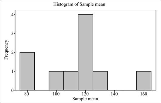
To graph: The histogram showing the 10 values of sample mean.

Explanation of Solution

The histogram showing the values of 10 sample mean is drawn in Minitab. The steps are written below:

Step 1. Enter the data in Minitab classifying the sample mean of 10 samples.

Step 2. Click on Graph in toolbox and click on histogram.

Step 3. Next, choose simple histogram option appearing in the dialog box and click OK.

Step 4. Drag the sample mean appearing on the left side in Graph variables and click on OK..

Graph: The obtained histogram showing the frequency and sample mean is as follows:

(d)

To determine

Whether the center of the histogram is close to population mean.

Answer to Problem 11E

Solution: The center of the histogram is close to population mean.

Explanation of Solution

The histogram drawn in part (c) shows that the sample means of 10 samples are close to 120 and the population mean computed in part (a) is equal to $120.5$. This shows that the population mean is approximately equal to the sample means obtained by drawing 10 simple random samples from the population.