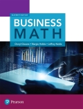
EBK BUSINESS MATH
11th Edition
ISBN: 8220103632072
Author: NOBLE
Publisher: Pearson Education (US)
expand_more
expand_more
format_list_bulleted
Concept explainers
Question
Chapter 5, Problem 5PT
To determine
To calculate: The solution of the equation
Expert Solution & Answer
Want to see the full answer?
Check out a sample textbook solution
Students have asked these similar questions
Using the method of sections need help solving this please explain im stuck
Find all the solutions of the congruence
7x² + 15x = 4 (mod 111).
) The set {1,2,..., 22} is to be split into two disjoint non-empty sets S
and T in such a way that:
(i) the product (mod 23) of any two elements of S lies in S;
(ii) the product (mod 23) of any two elements of T lies in S;
(iii) the product (mod 23) of any element of S and any element of T
lies in T.
Prove that the only solution is
S = {1, 2, 3, 4, 6, 8, 9, 12, 13, 16, 18},
T= {5, 7, 10, 11, 14, 15, 17, 19, 20, 21, 22}.
Chapter 5 Solutions
EBK BUSINESS MATH
Ch. 5.1 - Prob. 1-1SCCh. 5.1 - Prob. 1-2SCCh. 5.1 - Prob. 1-3SCCh. 5.1 - Prob. 1-4SCCh. 5.1 - Prob. 1-5SCCh. 5.1 - Prob. 1-6SCCh. 5.1 - Prob. 2-1SCCh. 5.1 - Prob. 2-2SCCh. 5.1 - Prob. 2-3SCCh. 5.1 - Prob. 2-4SC
Ch. 5.1 - Prob. 2-5SCCh. 5.1 - Prob. 2-6SCCh. 5.1 - Prob. 3-1SCCh. 5.1 - Prob. 3-2SCCh. 5.1 - Prob. 3-3SCCh. 5.1 - Prob. 3-4SCCh. 5.1 - Prob. 3-5SCCh. 5.1 - Prob. 3-6SCCh. 5.1 - Prob. 4-1SCCh. 5.1 - Prob. 4-2SCCh. 5.1 - Prob. 4-3SCCh. 5.1 - Prob. 4-4SCCh. 5.1 - Prob. 4-5SCCh. 5.1 - Prob. 4-6SCCh. 5.1 - Prob. 5-1SCCh. 5.1 - Prob. 5-2SCCh. 5.1 - Prob. 5-3SCCh. 5.1 - Prob. 5-4SCCh. 5.1 - Prob. 5-5SCCh. 5.1 - Prob. 5-6SCCh. 5.1 - Prob. 6-1SCCh. 5.1 - Prob. 6-2SCCh. 5.1 - Prob. 6-3SCCh. 5.1 - Prob. 6-4SCCh. 5.1 - Prob. 6-5SCCh. 5.1 - Prob. 6-6SCCh. 5.1 - Prob. 1SECh. 5.1 - Prob. 2SECh. 5.1 - Prob. 3SECh. 5.1 - Prob. 4SECh. 5.1 - Prob. 5SECh. 5.1 - Prob. 6SECh. 5.1 - Prob. 7SECh. 5.1 - Prob. 8SECh. 5.1 - Prob. 9SECh. 5.1 - Prob. 10SECh. 5.1 - Prob. 11SECh. 5.1 - Prob. 12SECh. 5.1 - Prob. 13SECh. 5.1 - Prob. 14SECh. 5.1 - Prob. 15SECh. 5.1 - Prob. 16SECh. 5.1 - Prob. 17SECh. 5.1 - Prob. 18SECh. 5.1 - Prob. 19SECh. 5.1 - Prob. 20SECh. 5.1 - Prob. 21SECh. 5.1 - Prob. 22SECh. 5.1 - Prob. 23SECh. 5.1 - Prob. 24SECh. 5.1 - Prob. 25SECh. 5.1 - Prob. 26SECh. 5.1 - Prob. 27SECh. 5.1 - Prob. 28SECh. 5.1 - Prob. 29SECh. 5.1 - Prob. 30SECh. 5.1 - Prob. 31SECh. 5.1 - Prob. 32SECh. 5.1 - Prob. 33SECh. 5.1 - Prob. 34SECh. 5.1 - Prob. 35SECh. 5.1 - Prob. 36SECh. 5.1 - Prob. 37SECh. 5.1 - Prob. 38SECh. 5.2 - Prob. 1-1SCCh. 5.2 - Prob. 1-2SCCh. 5.2 - Prob. 1-3SCCh. 5.2 - Prob. 1-4SCCh. 5.2 - Prob. 1-5SCCh. 5.2 - Prob. 1-6SCCh. 5.2 - Prob. 1SECh. 5.2 - Prob. 2SECh. 5.2 - Prob. 3SECh. 5.2 - Prob. 4SECh. 5.2 - Prob. 5SECh. 5.2 - Prob. 6SECh. 5.2 - Prob. 7SECh. 5.2 - Prob. 8SECh. 5.2 - Prob. 9SECh. 5.2 - Prob. 10SECh. 5.2 - Prob. 11SECh. 5.2 - Prob. 12SECh. 5.2 - Prob. 13SECh. 5.2 - Prob. 14SECh. 5.2 - Prob. 15SECh. 5.2 - Prob. 16SECh. 5.2 - Prob. 17SECh. 5.2 - Prob. 18SECh. 5.3 - Prob. 1-1SCCh. 5.3 - Prob. 1-2SCCh. 5.3 - Prob. 1-3SCCh. 5.3 - Prob. 1-4SCCh. 5.3 - Prob. 2-1SCCh. 5.3 - Prob. 2-2SCCh. 5.3 - Prob. 2-3SCCh. 5.3 - Prob. 2-4SCCh. 5.3 - Prob. 1SECh. 5.3 - Prob. 2SECh. 5.3 - Prob. 3SECh. 5.3 - Prob. 4SECh. 5.3 - Prob. 5SECh. 5.3 - Prob. 6SECh. 5.3 - Prob. 7SECh. 5.3 - Prob. 8SECh. 5.3 - Prob. 9SECh. 5.3 - Prob. 10SECh. 5.3 - Prob. 11SECh. 5.3 - Prob. 12SECh. 5.3 - Prob. 13SECh. 5.3 - Prob. 14SECh. 5.3 - Prob. 15SECh. 5.3 - Prob. 16SECh. 5 - Prob. 1ESCh. 5 - Prob. 2ESCh. 5 - Prob. 3ESCh. 5 - Prob. 4ESCh. 5 - Prob. 5ESCh. 5 - Prob. 6ESCh. 5 - Prob. 7ESCh. 5 - Prob. 8ESCh. 5 - Prob. 9ESCh. 5 - Prob. 10ESCh. 5 - Prob. 11ESCh. 5 - Prob. 12ESCh. 5 - Prob. 13ESCh. 5 - Prob. 14ESCh. 5 - Prob. 15ESCh. 5 - Prob. 16ESCh. 5 - Prob. 17ESCh. 5 - Prob. 18ESCh. 5 - Prob. 19ESCh. 5 - Prob. 20ESCh. 5 - Prob. 21ESCh. 5 - Prob. 22ESCh. 5 - Prob. 23ESCh. 5 - Prob. 24ESCh. 5 - Prob. 25ESCh. 5 - Prob. 26ESCh. 5 - Prob. 27ESCh. 5 - Prob. 28ESCh. 5 - Prob. 29ESCh. 5 - Prob. 30ESCh. 5 - Prob. 31ESCh. 5 - Prob. 32ESCh. 5 - Prob. 33ESCh. 5 - Prob. 34ESCh. 5 - Prob. 35ESCh. 5 - Prob. 36ESCh. 5 - Prob. 37ESCh. 5 - Prob. 38ESCh. 5 - Prob. 39ESCh. 5 - Prob. 40ESCh. 5 - Prob. 41ESCh. 5 - Prob. 42ESCh. 5 - Prob. 43ESCh. 5 - Prob. 44ESCh. 5 - Prob. 45ESCh. 5 - Prob. 46ESCh. 5 - Prob. 47ESCh. 5 - Prob. 48ESCh. 5 - Prob. 49ESCh. 5 - Prob. 50ESCh. 5 - Prob. 1PTCh. 5 - Prob. 2PTCh. 5 - Prob. 3PTCh. 5 - Prob. 4PTCh. 5 - Prob. 5PTCh. 5 - Prob. 6PTCh. 5 - Prob. 7PTCh. 5 - Prob. 8PTCh. 5 - Prob. 9PTCh. 5 - Prob. 10PTCh. 5 - Prob. 11PTCh. 5 - Prob. 12PTCh. 5 - Prob. 13PTCh. 5 - Prob. 14PTCh. 5 - Prob. 15PTCh. 5 - Prob. 16PTCh. 5 - Prob. 17PTCh. 5 - Prob. 18PTCh. 5 - Prob. 19PTCh. 5 - Prob. 20PTCh. 5 - Prob. 21PTCh. 5 - Prob. 1CTCh. 5 - Prob. 2CTCh. 5 - Prob. 3CTCh. 5 - Prob. 4CTCh. 5 - Prob. 5CTCh. 5 - Prob. 6CTCh. 5 - Prob. 7CTCh. 5 - Prob. 8CTCh. 5 - Prob. 1CPCh. 5 - Prob. 2CPCh. 5 - Prob. 1CS1Ch. 5 - Prob. 2CS1Ch. 5 - Prob. 3CS1Ch. 5 - Prob. 1CS2Ch. 5 - Prob. 2CS2Ch. 5 - Prob. 3CS2Ch. 5 - Prob. 4CS2Ch. 5 - Prob. 1CS3Ch. 5 - Prob. 2CS3Ch. 5 - Prob. 3CS3Ch. 5 - Prob. 4CS3
Knowledge Booster
Learn more about
Need a deep-dive on the concept behind this application? Look no further. Learn more about this topic, subject and related others by exploring similar questions and additional content below.Similar questions
- 19) Consider this initial value problem: y' + y = 2y = -21² + 2t+ 14, y(0) = 0, y (0) = 0 - What is the solution of the initial value problem?arrow_forward4) Consider the initial value problem " 8y +30y+25y = 0, y(0) = -2, y (0) = 8 What is the t-coordinate of the local extreme value of y = y(t) on the interval (0, ∞)? Enter your answer as a decimal accurate to three decimal places.arrow_forwardTips S ps L 50. lim x2 - 4 x-2x+2 51. lim 22 - X 52. 53. x 0 Answer lim x 0 lim 2-5 X 2x2 2 x² Answer -> 54. lim T - 3x - - 25 +5 b+1 b3b+3 55. lim X x-1 x 1 Answer 56. lim x+2 x 2 x 2 57. lim x²-x-6 x-2 x²+x-2 Answer-> 23-8 58. lim 2-22-2arrow_forward
- 10) Which of the following is the general solution of the homogeneous second-order differential equation y + 8y + 52y=0? Here, C, C₁, and C2 are arbitrary real constants. A) y = C₁ecos(61) + C₂e*sin(61) + C B) y = et (sin(4t) + cos(6t)) + C C) y = C₁esin(6) + C₂e+ cos(6t) + C D) y = C₁esin(6) + C₂e+cos(6) E) y=e(C₁sin(61) + C₂cos(61))arrow_forward3) Consider the initial value problem ' y' + 8y = 0, y(0) = -4, y (0) = 16 What is the solution of this initial value problem? A) y = -4t - 2e8t D) y = -4 + 2e-8t B) y = -2 + 2e8t C) y = -2 -2e-8t E) y = -4+ 2e8t F) y = -2t-2e-8tarrow_forward6) Consider the initial value problem y + cos πι + e²бty = 0, y(-1) = 0, y' (-1) = 0 Which of these statements are true? Select all that apply. A) There exists a nonzero real number r such that y(t) = ert is a solution of the initial value problem. B) The constant function y(t) = -1 is a solution of this initial value problem for all real numbers t. C) The constant function y(t) = 0 is the unique solution of this initial value problem on the interval (-∞, ∞). D) This initial value problem has only one solution on the interval (-7, 5). E) There must exist a function y = q(t) that satisfies this initial value problem on the interval (-7,∞).arrow_forward
- 7) Compute the Wronskian of the pair of functions sin(5t) and cos(5t). A) -5 B) 4 C) 1 D) -4 E) 5arrow_forward8) The pair of functions y₁ = eбt and y₁ = teбt forms a fundamental set of solutions for the differential equation y'' - 12y' + 36y= 0.arrow_forward6) Consider the initial value problem y + cos πι + e²бty = 0, y(-1) = 0, y' (-1) = 0 Which of these statements are true? Select all that apply. A) There exists a nonzero real number r such that y(t) = ert is a solution of the initial value problem. B) The constant function y(t) = -1 is a solution of this initial value problem for all real numbers t. C) The constant function y(t) = 0 is the unique solution of this initial value problem on the interval (-∞, ∞). D) This initial value problem has only one solution on the interval (-7, 5). E) There must exist a function y = q(t) that satisfies this initial value problem on the interval (-7,∞).arrow_forward
arrow_back_ios
SEE MORE QUESTIONS
arrow_forward_ios
Recommended textbooks for you
 Discrete Mathematics and Its Applications ( 8th I...MathISBN:9781259676512Author:Kenneth H RosenPublisher:McGraw-Hill Education
 Mathematics for Elementary Teachers with Activiti...MathISBN:9780134392790Author:Beckmann, SybillaPublisher:PEARSON
 Thinking Mathematically (7th Edition)MathISBN:9780134683713Author:Robert F. BlitzerPublisher:PEARSON
 Discrete Mathematics With ApplicationsMathISBN:9781337694193Author:EPP, Susanna S.Publisher:Cengage Learning,
 Pathways To Math Literacy (looseleaf)MathISBN:9781259985607Author:David Sobecki Professor, Brian A. MercerPublisher:McGraw-Hill Education

Discrete Mathematics and Its Applications ( 8th I...
Math
ISBN:9781259676512
Author:Kenneth H Rosen
Publisher:McGraw-Hill Education

Mathematics for Elementary Teachers with Activiti...
Math
ISBN:9780134392790
Author:Beckmann, Sybilla
Publisher:PEARSON


Thinking Mathematically (7th Edition)
Math
ISBN:9780134683713
Author:Robert F. Blitzer
Publisher:PEARSON

Discrete Mathematics With Applications
Math
ISBN:9781337694193
Author:EPP, Susanna S.
Publisher:Cengage Learning,

Pathways To Math Literacy (looseleaf)
Math
ISBN:9781259985607
Author:David Sobecki Professor, Brian A. Mercer
Publisher:McGraw-Hill Education
Statistics 4.1 Introduction to Inferential Statistics; Author: Dr. Jack L. Jackson II;https://www.youtube.com/watch?v=QLo4TEvBvK4;License: Standard YouTube License, CC-BY