a.
To calculate: Future value of $1,000 after 5 years at 10% annual interest rate.
Introduction:
a.
Explanation of Solution
Calculation in spreadsheet by “FV” formula,
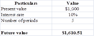
Table (1)
Steps required to calculate present value by using “FV” function in excel are given,
- Select ‘Formulas’ option from Menu Bar of Excel sheet.
- Select insert Function that is (fx).
- Choose category of Financial.
- Then select “FV” and then press OK.
- A window will pop up.
- Input data in the required field.
- Final answer will be shown by the formula that is $1,610.50.
Future value of $1,000 is $1,610.51.
b.
To calculate: Investments future value at 0%,5% and 20% rate after 0,1,2,3,4 and 5 years.
Introduction:
Time Value of Money: It is a vital concept to the investors, as it suggests them the money they are having today is worth more than the value promised in the future.
b.
Explanation of Solution
Calculation spreadsheet by “FV” formula,

Table (2)
Steps required to calculate present value by using “FV” function in excel are given,
- Select ‘Formulas’ option from Menu Bar of Excel sheet.
- Select insert Function that is (fx).
- Choose category of Financial.
- Then select “FV” and then press OK.
- A window will pop up.
- Input data in required field.
Investment future values are different for the different years with 0%, 5% and 20% interest rate.
c.
To calculate: Present value due of $1,000 in 5 years at the discount rate of 10%.
Introduction:
Time Value of Money: It is a vital concept to the investors, as it suggests them the money they are having today is worth more than the value promised in the future.
c.
Explanation of Solution
Calculation in spreadsheet by “PV” formula,
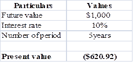
Table (3)
Steps required to calculate present value by using “PV” function in excel are given,
- Select ‘Formulas’ option from Menu Bar of Excel sheet.
- Select insert Function that is (fx).
- Choose category of Financial.
- Then select “PV” and then press OK.
- A window will pop up.
- Input data in the required field.
- Final answer will be shown by the formula that is $620.92.
Present value of $1,000 is $620.92 at 10 % discount rate.
d.
To calculate:
Introduction:
Time Value of Money: It is a vital concept to the investors, as it suggests them the money they are having today is worth more than the value promised in the future.
d.
Explanation of Solution
Calculationin spreadsheet by “RATE” formula,
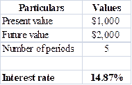
Table (4)
Steps required to calculate present value by using “RATE” function in excel are given,
- Select ‘Formulas’ option from Menu Bar of Excel sheet.
- Select insert Function that is (fx).
- Choose category of Financial.
- Then select “RATE” and then press OK.
- A window will pop up.
- Input data in the required field.
- Final answer will be shown by the formula that is 14.87%
The rate of return is14.87%.
e.
To calculate: Time taken by 36.5 million populations to double with annual growth rate of 2%
Introduction:
Time Value of Money: It is a vital concept to the investors, as it suggests them the money they are having today is worth more than the value promised in the future.
e.
Explanation of Solution
Calculation is solved in spreadsheet by “NPER” formula
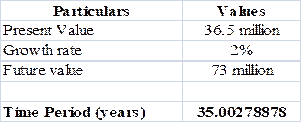
Table (5)
Steps required to calculate present value by using “NPER” function in excel are given,
- Select ‘Formulas’ option from Menu Bar of excel sheet.
- Select insert Function that is (fx).
- Choose category of Financial.
- Then select “NPER” and then press OK.
- A window will pop up.
- Input data in the required field.
- Final answer will be shown by the formula that is 35 years.
Conclusion:
It will take 35 years to double the population from 36.5 million to 73 million.
f.
To calculate: Present and future value of
Introduction:
Time Value of Money: It is a vital concept to the investors, as it suggests them the money they are having today is worth more than the value promised in the future.
f.
Explanation of Solution
Calculation in spreadsheet by “PV” formula,
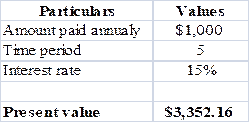
Table (6)
Steps required to calculate present value by using “PV” function in excel are given,
- Select ‘Formulas’ option from Menu Bar of Excel sheet.
- Select insert Function that is (fx).
- Choose category of Financial.
- Then select “PV” and then press OK.
- A window will pop up.
- Input data in the required field.
- Final answer will be shown by the formula that is $3,352.16.
So, the present value is $3,352.16.
Calculation of future value of
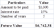
Table (7)
Steps required to calculate present value by using “FV” function in excel are given,
- Select ‘Formulas’ option from Menu Bar of Excel sheet.
- Select insert Function that is (fx).
- Choose category of Financial.
- Then select “FV” and then press OK.
- A window will pop up.
- Input data in the required field.
- Final answer will be shown by the formula that is $6,742.38.
So the future value is $6,742.38.
Present value is $3,352.16 and future value is $6,742.38 of
g.
To calculate: Present and future value of part ‘f’ if the
Introduction:
Time Value of Money: It is a vital concept to the investors, as it suggests them the money they are having today is worth more than the value promised in the future.
g.
Explanation of Solution
Calculation in spreadsheet by “PV” function,
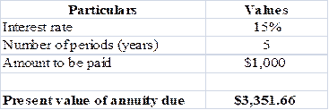
Table (8)
Steps required to calculate present value by using “PV” function in excel are given,
- Select ‘Formulas’ option from Menu Bar of Excel sheet.
- Select insert Function that is (fx).
- Choose category of Financial.
- Then select “PV” and then press OK.
- A window will pop up.
- Input data in the required field.
- Final answer will be shown by the formula that is $3,351.66.
Present value of
Future value of annuity in spreadsheet by “FV” function,
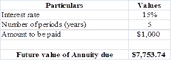
Table (9)
Steps required to calculate present value by using “FV” function in excel are given,
- Select ‘Formulas’ option from Menu Bar of Excel sheet.
- Select insert Function that is (fx).
- Choose category of Financial.
- Then select “FV” and then press OK.
- A window will pop up.
- Input data in the required field.
- Final answer will be shown by the formula that is $7,753.74
Future value of annuity due is $7,753.74.
Present value of
h.
To calculate: Present and future value for $1,000, due in 5 years with 10% semiannual compounding.
Introduction:
Time Value of Money: It is a vital concept to the investors, as it suggests them the money they are having today is worth more than the value promised in the future.
h.
Explanation of Solution
Calculation in spreadsheet by “PV” formula,

Table (10)
Steps required to calculate present value by using “PV” function in excel are given,
- Select ‘Formulas’ option from Menu Bar of Excel sheet.
- Select insert Function that is (fx).
- Choose category of Financial.
- Then select “PV” and then press OK.
- A window will pop up.
- Input data in the required field.
- Final answer will be shown by the formula that is $613.91.
Present value is $613.91.
Calculation in spreadsheet by “FV” formula,
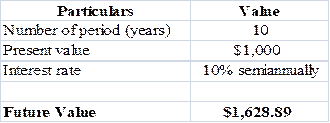
Table (11)
Steps required to calculate present value by using “FV” function in excel are given,
- Select ‘Formulas’ option from Menu Bar of Excel sheet.
- Select insert Function that is (fx).
- Choose category of Financial.
- Then select “FV” and then press OK.
- A window will pop up.
- Input data in the required field.
- Final answer will be shown by the formula that is $1,628.89.
Future value of
Present andfuture value for $1,000, due in 5 years with 10% semiannual compoundingwill be $613.91 and $1,628.89, respectively.
i.
To calculate: Annual payments for an ordinary
Introduction:
Time Value of Money: It is a vital concept to the investors, as it suggests them the money they are having today is worth more than the value promised in the future.
i.
Explanation of Solution
Calculation in spreadsheet by “PMT” formula,
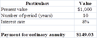
Table (12)
Steps required to calculate present value by using “PMT” function in excel are given,
- Select ‘Formulas’ option from Menu Bar of Excel sheet.
- Select insert Function that is (fx).
- Choose category of Financial.
- Then select “PMT” and then press OK.
- A window will pop up.
- Input data in the required field.
- Final answer will be shown by the formula that is $1,628.89.
Payment of ordinary
Calculation in spreadsheet by “PMT” formula,
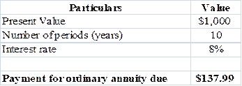
Table (13)
Steps required to calculate present value by using “PMT” function in excel are given,
- Select ‘Formulas’ option from Menu Bar of Excel sheet.
- Select insert Function that is (fx).
- Choose category of Financial.
- Then select “PMT” and then press OK.
- A window will pop up.
- Input data in the required field.
- Final answer will be shown by the formula that is $1,628.89.
Payment of ordinary annuity due is $137.99.
Annual payments are$149.03 for an ordinary
j.
To calculate: Present value and future value of an investment that pays 8% annually and makes the year end payments of $100, $200,$300.
j.
Explanation of Solution
Calculation in spreadsheet by “
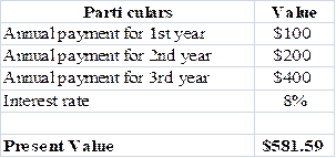
Table (14)
Steps required to calculate present value by using “NPV” function in excel are given,
- Select ‘Formulas’ option from Menu Bar of Excel sheet.
- Select insert Function that is (fx).
- Choose category of Financial.
- Then select “NPV” and then press OK.
- A window will pop up.
- Input data in the required field.
- Final answer will be shown by the formula that is $581.59.
Present value is $581.59.
Calculation in spreadsheet by “FV” formula,
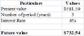
Table (15)
Steps required to calculate present value by using “FV” function in excel are given,
- Select ‘Formulas’ option from Menu Bar of Excel sheet.
- Select insert Function that is (fx).
- Choose category of Financial.
- Then select “FV” and then press OK.
- A window will pop up.
- Input data in the required field.
- Final answer will be shown by the formula that is $732.54.
Future value is $732.54.
Present value is $581.89 while future value is $732.54.
k.1.
To calculate: Effective annual rate each bank pays and the future value of $5,000 at the end of 1 and 2 year.
k.1.
Explanation of Solution
Given for Bank A,
Nominal interest rate is 5%.
Compounding is annual.
Formula to calculate effective annual rate is,
Where,
- EFF is the effective annual rate.
- INOM is the nominal interest rate.
- M is the compounding period.
Substitute 5% for INOM and 1 for M.
So, effective annual rate for Bank A is 5%.
Given for Bank B,
Nominal interest rate is 5%.
Compounding is semiannual.
Formula to calculate effective annual rate is,
Where,
- EFF is the effective annual rate.
- INOM is the nominal interest rate.
- M is the compounding period.
Substitute 5% for INOM and 2 for M.
So,effective annual rate for Bank B is 5.06%.
Given for Bank C,
Nominal interest rate is 5%.
Compounding is quarterly.
Formula to calculate effective annual rate is,
Where,
- EFF is the effective annual rate.
- INOM is the nominal interest rate.
- M is the compounding period.
Substitute 5% for INOM and 4 for M.
So, effective annual rate for Bank C is 5.09%.
Given for Bank D,
Nominal interest rate is 5%.
Compounding ismonthly.
Formula to calculate effective annual rate is,
Where,
- EFF is the effective annual rate.
- INOM is the nominal interest rate.
- M is the compounding period.
Substitute 5% for INOM and 12 for M.
So, effective annual rate for Bank D is 5.11%.
Given for Bank E,
Nominal interest rate is 5%.
Compounding is daily.
Formula to calculate effective annual rate is,
Where,
- EFF is the effective annual rate.
- INOM is the nominal interest rate.
- M is the compounding period.
Substitute 5% for INOM and 365 for M.
So, effective annual rate for Bank E is 5.12%.
Calculation of future value in spreadsheet by “FV” formula,

Table (16)
Steps required to calculate present value by using “FV” function in excel are given,
- Select ‘Formulas’ option from Menu Bar of Excel sheet.
- Select insert Function that is (fx).
- Choose category of Financial.
- Then select “FV” and then press OK.
- A window will pop up.
- Input data in the required field.
So, the future value at different effective rate after a year are $5, 250, $5,253,$5,254.50, $5,255.50 and $5,256.
Calculation of future value in spreadsheet by “FV” formula,

Table (17)
Steps required to calculate present value by using “FV” function in excel are given,
- Select ‘Formulas’ option from Menu Bar of Excel sheet.
- Select insert Function that is (fx).
- Choose category of Financial.
- Then select “FV” and then press OK.
- A window will pop up.
- Input data in the required field.
So, the future value at different effective rate after a year are $5, 512, $5,518.80, $5,521.95, $5,524.06 and $5,525.11.
Each bank pays different effective rate as there compounding is different, the rates are5% for bank A, 5.06% Bank B, 5.09% Bank C, 5.11% Bank D, 5.12% Bank E, also the future values also change on the basis of their number of periods.
2.
To explain: If banks are insured by the government and are equally risky, will they be equally able to attract funds and at what nominal rate all banks provide equal effective rate as Bank A.
2.
Answer to Problem 41SP
No, it is not possible for the banks to equally attract funds.
The nominal rate which causes same effective rate for all banks are,
| Particulars | A | B | C | D | E |
| Nominalrate | 5% | 5.06% | 5.09% | 5.11% | 5.12% |
Table (18)
Explanation of Solution
- Bank will not be equally able to attract funds because of compounding, as people prefer to invest in that bank which have more frequent compounding in comparison to the bank which have lesser frequent compounding.
- Nominal rate is opposite of the effective rate which is calculated in part ‘1’. The nominal rate indicated in above table will cause same effective rate for all banks as it is for A bank.
Due to frequent compounding, banks will not be able to equally attract funds and the nominal rate will be 5% for Bank A, 5.06% Bank B, 5.09% Bank C, 5.11% Bank D, 5.12% Bank E.
3.
To calculate: Present value of amount to get $5,000 after 1 year.
3.
Explanation of Solution
Calculation of payment to be made in spreadsheet by “PMT” formula,

Table (19)
Steps required to calculate present value by using “PMT” function in excel are given,
- Select ‘Formulas’ option from Menu Bar of Excel sheet.
- Select insert Function that is (fx).
- Choose category of Financial.
- Then select “PMT” and then press OK.
- A window will pop up.
- Input data in the required field.
So, the amounts to be paid are$4,761.90,$2498.10,$1,102.40,$296.96 and $15.83.
4.
To explain: If all banks are providing a same effective interest rate would rational investor be indifferent between the banks.
4.
Answer to Problem 41SP
Yes, a rational investor would be indifferent between the banks.
Explanation of Solution
Rational investor chooses the bank which will provide him better return so he would be indifferent, if all the banks are giving same effective rate because he chooses the bank which will have more frequent compounding than others.
A bank offers frequent compounding is able to attract more number of customers than others.
To prepare: Amortization schedule to show annual payments, interest payments, principal payments, and beginning and ending loan balances.
Amortization:
Amotization means to write off or pay the debt over the priod of time it can be for loan or intangible assets. Its main purpose is to get cost recovery. Example of amortization is ,an automobile company that spent $20 million dollars on a design patent with a useful life of 20 years. The amortization value for that company will be $1 million each year.
Explanation of Solution
Calculation of annual installment is done by using “PMT” formula in spreadsheet at the amortization schedule.
Amortization schedule is prepared below,

Table (20)
Steps required to calculate present value by using “PMT” function in excel are given,
- Select ‘Formulas’ option from Menu Bar of Excel sheet.
- Select insert Function that is (fx).
- Choose category of Financial.
- Then select “PMT” and then press OK.
- A window will pop up.
- Input data in the required field.
Amortization schedule represents annual payments, interest payments, principal payments, and beginning and ending loan balances.
Want to see more full solutions like this?
Chapter 5 Solutions
Fundamentals of Financial Management (MindTap Course List)
- Describe in detail what exactly is the Cash Conversion Cycle, how is it computed and what is the purpose of this calculation (how is it used).arrow_forwardExplain what Interest Rate Parity is, how it is calculated, and why it is important to a company operating internationally.arrow_forwardCompare and contrast the three core means of adding shareholder wealth; Cash Dividends, Stock Dividends and Stock Splits, and Stock Repurchases. Include the various advantages and disadvantages of each one.arrow_forward
- Calculate the future value of a lump sum of $1,000 invested for 4 years at 10%, using compounded quarterly.arrow_forwardIf value is not clear then please comment i will write values dont solve question, i will give unhelpful.arrow_forwardwhat are some of the question can i asek my prinsiple of finance teache?arrow_forward
- A critical discussion of the hockey stick model of start-up financing should be presented, supported by recent in-text citations. Provide a detailed explanation of the model. Describe each of the three stages of the hockey stick model of start-up financing, including a detailed characterisation of each stage. The characterisation of each stage should detail the growth, risk, and funding expectations. Present a critical evaluation and an insightful conclu sion.arrow_forwardQuestion Workspace Check My Work New-Project Analysis The president of your company, MorChuck Enterprises, has asked you to evaluate the proposed acquisition of a new chromatograph for the firm's R&D department. The equipment's basic price is $64,000, and it would cost another $18,000 to modify it for special use by your firm. The chromatograph, which falls into the MACRS 3-year class, would be sold after 3 years for $28,400. The MACRS rates for the first three years are 0.3333, 0.4445 and 0.1481. (Ignore the half-year convention for the straight-line method.) Use of the equipment would require an increase in net working capital (spare parts inventory) of $3,000. The machine would have no effect on revenues, but it is expected to save the firm $24,760 per year in before-tax operating costs, mainly labor. The firm's marginal federal-plus-state tax rate is 25%. Cash outflows and negative NPV value, if any, should be indicated by a minus sign. Do not round intermediate…arrow_forwardAlthough the Chen Company's milling machine is old, it is still in relatively good working order and would last for another 10 years. It is inefficient compared to modern standards, though, and so the company is considering replacing it. The new milling machine, at a cost of $108,000 delivered and installed, would also last for 10 years and would produce after-tax cash flows (labor savings and depreciation tax savings) of $19,000 per year. It would have zero salvage value at the end of its life. The project cost of capital is 11%, and its marginal tax rate is 25%. Should Chen buy the new machine? Do not round intermediate calculations. Round your answer to the nearest cent. Negative value, if any, should be indicated by a minus sign.arrow_forward
 Essentials Of InvestmentsFinanceISBN:9781260013924Author:Bodie, Zvi, Kane, Alex, MARCUS, Alan J.Publisher:Mcgraw-hill Education,

 Foundations Of FinanceFinanceISBN:9780134897264Author:KEOWN, Arthur J., Martin, John D., PETTY, J. WilliamPublisher:Pearson,
 Fundamentals of Financial Management (MindTap Cou...FinanceISBN:9781337395250Author:Eugene F. Brigham, Joel F. HoustonPublisher:Cengage Learning
 Corporate Finance (The Mcgraw-hill/Irwin Series i...FinanceISBN:9780077861759Author:Stephen A. Ross Franco Modigliani Professor of Financial Economics Professor, Randolph W Westerfield Robert R. Dockson Deans Chair in Bus. Admin., Jeffrey Jaffe, Bradford D Jordan ProfessorPublisher:McGraw-Hill Education

