a.
To calculate: Future value of $1,000 after 5 years at 10% annual interest rate.
Introduction:
a.
Explanation of Solution
Calculation in spreadsheet by “FV” formula,
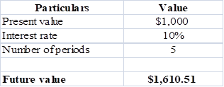
Table (1)
Steps required to calculate
- Select ‘Formulas’ option from Menu Bar of Excel sheet.
- Select insert Function that is (fx).
- Choose category of Financial.
- Then select “FV” and then press OK.
- A window will pop up.
- Input data in the required field.
- Final answer will be shown by the formula that is $1,610.50.
Future value of $1,000 is $1,610.51.
b.
To calculate: Investments future value at 0%,5% and 20% rate after 0,1,2,3,4 and 5 years.
Introduction:
Time Value of Money: It is a vital concept to the investors, as it suggests them the money they are having today is worth more than the value promised in the future.
b.
Explanation of Solution
Calculation spreadsheet by “FV” formula,
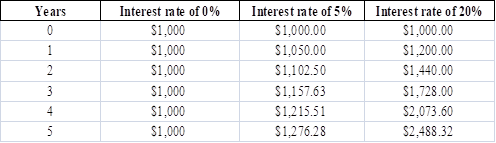
Table (2)
Steps required to calculate present value by using “FV” function in excel are given,
- Select ‘Formulas’ option from Menu Bar of Excel sheet.
- Select insert Function that is (fx).
- Choose category of Financial.
- Then select “FV” and then press OK.
- A window will pop up.
- Input data in required field.
Investment future values are different for the different years with 0%, 5% and 20% interest rate.
c.
To calculate: Present value due of $1,000 in 5 years at the discount rate of 10%.
Introduction:
Time Value of Money: It is a vital concept to the investors, as it suggests them the money they are having today is worth more than the value promised in the future.
c.
Explanation of Solution
Calculation in spreadsheet by “PV” formula,
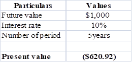
Table (3)
Steps required to calculate present value by using “PV” function in excel are given,
- Select ‘Formulas’ option from Menu Bar of Excel sheet.
- Select insert Function that is (fx).
- Choose category of Financial.
- Then select “PV” and then press OK.
- A window will pop up.
- Input data in the required field.
- Final answer will be shown by the formula that is $620.92.
Present value of $1,000 is $620.92 at 10 % discount rate.
d.
To calculate:
Introduction:
Time Value of Money: It is a vital concept to the investors, as it suggests them the money they are having today is worth more than the value promised in the future.
d.
Explanation of Solution
Calculationin spreadsheet by “RATE” formula,
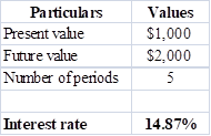
Table (4)
Steps required to calculate present value by using “RATE” function in excel are given,
- Select ‘Formulas’ option from Menu Bar of Excel sheet.
- Select insert Function that is (fx).
- Choose category of Financial.
- Then select “RATE” and then press OK.
- A window will pop up.
- Input data in the required field.
- Final answer will be shown by the formula that is 14.87%
The rate of return is14.87%.
e.
To calculate: Time taken by 36.5 million populations to double with annual growth rate of 2%
Introduction:
Time Value of Money: It is a vital concept to the investors, as it suggests them the money they are having today is worth more than the value promised in the future.
e.
Explanation of Solution
Calculation is solved in spreadsheet by “NPER” formula
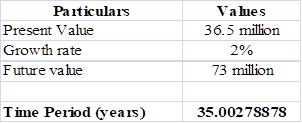
Table (5)
Steps required to calculate present value by using “NPER” function in excel are given,
- Select ‘Formulas’ option from Menu Bar of excel sheet.
- Select insert Function that is (fx).
- Choose category of Financial.
- Then select “NPER” and then press OK.
- A window will pop up.
- Input data in the required field.
- Final answer will be shown by the formula that is 35 years.
Conclusion:
It will take 35 years to double the population from 36.5 million to 73 million.
f.
To calculate: Present and future value of
Introduction:
Time Value of Money: It is a vital concept to the investors, as it suggests them the money they are having today is worth more than the value promised in the future.
f.
Explanation of Solution
Calculation in spreadsheet by “PV” formula,
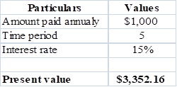
Table (6)
Steps required to calculate present value by using “PV” function in excel are given,
- Select ‘Formulas’ option from Menu Bar of Excel sheet.
- Select insert Function that is (fx).
- Choose category of Financial.
- Then select “PV” and then press OK.
- A window will pop up.
- Input data in the required field.
- Final answer will be shown by the formula that is $3,352.16.
So, the present value is $3,352.16.
Calculation of future value of
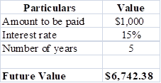
Table (7)
Steps required to calculate present value by using “FV” function in excel are given,
- Select ‘Formulas’ option from Menu Bar of Excel sheet.
- Select insert Function that is (fx).
- Choose category of Financial.
- Then select “FV” and then press OK.
- A window will pop up.
- Input data in the required field.
- Final answer will be shown by the formula that is $6,742.38.
So the future value is $6,742.38.
Present value is $3,352.16 and future value is $6,742.38 of
g.
To calculate: Present and future value of part ‘f’ if the
Introduction:
Time Value of Money: It is a vital concept to the investors, as it suggests them the money they are having today is worth more than the value promised in the future.
g.
Explanation of Solution
Calculation in spreadsheet by “PV” function,
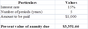
Table (8)
Steps required to calculate present value by using “PV” function in excel are given,
- Select ‘Formulas’ option from Menu Bar of Excel sheet.
- Select insert Function that is (fx).
- Choose category of Financial.
- Then select “PV” and then press OK.
- A window will pop up.
- Input data in the required field.
- Final answer will be shown by the formula that is $3,351.66.
Present value of
Future value of annuity in spreadsheet by “FV” function,
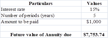
Table (9)
Steps required to calculate present value by using “FV” function in excel are given,
- Select ‘Formulas’ option from Menu Bar of Excel sheet.
- Select insert Function that is (fx).
- Choose category of Financial.
- Then select “FV” and then press OK.
- A window will pop up.
- Input data in the required field.
- Final answer will be shown by the formula that is $7,753.74
Future value of annuity due is $7,753.74.
Present value of
h.
To calculate: Present and future value for $1,000, due in 5 years with 10% semiannual compounding.
Introduction:
Time Value of Money: It is a vital concept to the investors, as it suggests them the money they are having today is worth more than the value promised in the future.
h.
Explanation of Solution
Calculation in spreadsheet by “PV” formula,
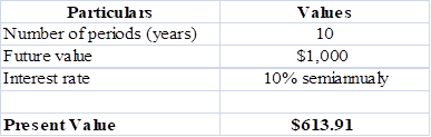
Table (10)
Steps required to calculate present value by using “PV” function in excel are given,
- Select ‘Formulas’ option from Menu Bar of Excel sheet.
- Select insert Function that is (fx).
- Choose category of Financial.
- Then select “PV” and then press OK.
- A window will pop up.
- Input data in the required field.
- Final answer will be shown by the formula that is $613.91.
Present value is $613.91.
Calculation in spreadsheet by “FV” formula,
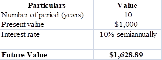
Table (11)
Steps required to calculate present value by using “FV” function in excel are given,
- Select ‘Formulas’ option from Menu Bar of Excel sheet.
- Select insert Function that is (fx).
- Choose category of Financial.
- Then select “FV” and then press OK.
- A window will pop up.
- Input data in the required field.
- Final answer will be shown by the formula that is $1,628.89.
Future value of
Present andfuture value for $1,000, due in 5 years with 10% semiannual compoundingwill be $613.91 and $1,628.89, respectively.
i.
To calculate: Annual payments for an ordinary
Introduction:
Time Value of Money: It is a vital concept to the investors, as it suggests them the money they are having today is worth more than the value promised in the future.
i.
Explanation of Solution
Calculation in spreadsheet by “PMT” formula,
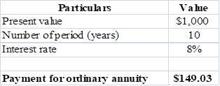
Table (12)
Steps required to calculate present value by using “PMT” function in excel are given,
- Select ‘Formulas’ option from Menu Bar of Excel sheet.
- Select insert Function that is (fx).
- Choose category of Financial.
- Then select “PMT” and then press OK.
- A window will pop up.
- Input data in the required field.
- Final answer will be shown by the formula that is $1,628.89.
Payment of ordinary
Calculation in spreadsheet by “PMT” formula,
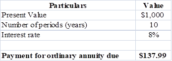
Table (13)
Steps required to calculate present value by using “PMT” function in excel are given,
- Select ‘Formulas’ option from Menu Bar of Excel sheet.
- Select insert Function that is (fx).
- Choose category of Financial.
- Then select “PMT” and then press OK.
- A window will pop up.
- Input data in the required field.
- Final answer will be shown by the formula that is $1,628.89.
Payment of ordinary annuity due is $137.99.
Annual payments are$149.03 for an ordinary
j.
To calculate: Present value and future value of an investment that pays 8% annually and makes the year end payments of $100, $200,$300.
j.
Explanation of Solution
Calculation in spreadsheet by “
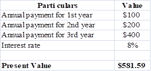
Table (14)
Steps required to calculate present value by using “NPV” function in excel are given,
- Select ‘Formulas’ option from Menu Bar of Excel sheet.
- Select insert Function that is (fx).
- Choose category of Financial.
- Then select “NPV” and then press OK.
- A window will pop up.
- Input data in the required field.
- Final answer will be shown by the formula that is $581.59.
Present value is $581.59.
Calculation in spreadsheet by “FV” formula,
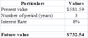
Table (15)
Steps required to calculate present value by using “FV” function in excel are given,
- Select ‘Formulas’ option from Menu Bar of Excel sheet.
- Select insert Function that is (fx).
- Choose category of Financial.
- Then select “FV” and then press OK.
- A window will pop up.
- Input data in the required field.
- Final answer will be shown by the formula that is $732.54.
Future value is $732.54.
Present value is $581.89 while future value is $732.54.
k.1.
To calculate: Effective annual rate each bank pays and the future value of $5,000 at the end of 1 and 2 year.
k.1.
Explanation of Solution
Given for Bank A,
Nominal interest rate is 5%.
Compounding is annual.
Formula to calculate effective annual rate is,
Where,
- EFF is the effective annual rate.
- INOM is the nominal interest rate.
- M is the compounding period.
Substitute 5% for INOM and 1 for M.
So, effective annual rate for Bank A is 5%.
Given for Bank B,
Nominal interest rate is 5%.
Compounding is semiannual.
Formula to calculate effective annual rate is,
Where,
- EFF is the effective annual rate.
- INOM is the nominal interest rate.
- M is the compounding period.
Substitute 5% for INOM and 2 for M.
So,effective annual rate for Bank B is 5.06%.
Given for Bank C,
Nominal interest rate is 5%.
Compounding is quarterly.
Formula to calculate effective annual rate is,
Where,
- EFF is the effective annual rate.
- INOM is the nominal interest rate.
- M is the compounding period.
Substitute 5% for INOM and 4 for M.
So, effective annual rate for Bank C is 5.09%.
Given for Bank D,
Nominal interest rate is 5%.
Compounding ismonthly.
Formula to calculate effective annual rate is,
Where,
- EFF is the effective annual rate.
- INOM is the nominal interest rate.
- M is the compounding period.
Substitute 5% for INOM and 12 for M.
So, effective annual rate for Bank D is 5.11%.
Given for Bank E,
Nominal interest rate is 5%.
Compounding is daily.
Formula to calculate effective annual rate is,
Where,
- EFF is the effective annual rate.
- INOM is the nominal interest rate.
- M is the compounding period.
Substitute 5% for INOM and 365 for M.
So, effective annual rate for Bank E is 5.12%.
Calculation of future value in spreadsheet by “FV” formula,
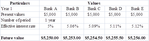
Table (16)
Steps required to calculate present value by using “FV” function in excel are given,
- Select ‘Formulas’ option from Menu Bar of Excel sheet.
- Select insert Function that is (fx).
- Choose category of Financial.
- Then select “FV” and then press OK.
- A window will pop up.
- Input data in the required field.
So, the future value at different effective rate after a year are $5, 250, $5,253,$5,254.50, $5,255.50 and $5,256.
Calculation of future value in spreadsheet by “FV” formula,
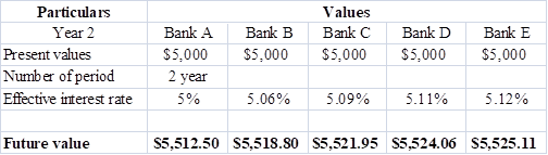
Table (17)
Steps required to calculate present value by using “FV” function in excel are given,
- Select ‘Formulas’ option from Menu Bar of Excel sheet.
- Select insert Function that is (fx).
- Choose category of Financial.
- Then select “FV” and then press OK.
- A window will pop up.
- Input data in the required field.
So, the future value at different effective rate after a year are $5, 512, $5,518.80, $5,521.95, $5,524.06 and $5,525.11.
Each bank pays different effective rate as there compounding is different, the rates are5% for bank A, 5.06% Bank B, 5.09% Bank C, 5.11% Bank D, 5.12% Bank E, also the future values also change on the basis of their number of periods.
2.
To explain: If banks are insured by the government and are equally risky, will they be equally able to attract funds and at what nominal rate all banks provide equal effective rate as Bank A.
2.
Answer to Problem 41SP
No, it is not possible for the banks to equally attract funds.
The nominal rate which causes same effective rate for all banks are,
| Particulars | A | B | C | D | E |
| Nominalrate | 5% | 5.06% | 5.09% | 5.11% | 5.12% |
Table (18)
Explanation of Solution
- Bank will not be equally able to attract funds because of compounding, as people prefer to invest in that bank which have more frequent compounding in comparison to the bank which have lesser frequent compounding.
- Nominal rate is opposite of the effective rate which is calculated in part ‘1’. The nominal rate indicated in above table will cause same effective rate for all banks as it is for A bank.
Due to frequent compounding, banks will not be able to equally attract funds and the nominal rate will be 5% for Bank A, 5.06% Bank B, 5.09% Bank C, 5.11% Bank D, 5.12% Bank E.
3.
To calculate: Present value of amount to get $5,000 after 1 year.
3.
Explanation of Solution
Calculation of payment to be made in spreadsheet by “PMT” formula,
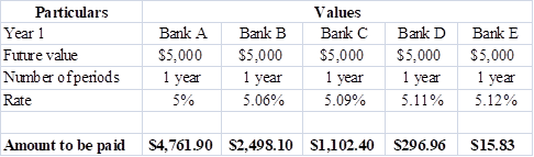
Table (19)
Steps required to calculate present value by using “PMT” function in excel are given,
- Select ‘Formulas’ option from Menu Bar of Excel sheet.
- Select insert Function that is (fx).
- Choose category of Financial.
- Then select “PMT” and then press OK.
- A window will pop up.
- Input data in the required field.
So, the amounts to be paid are$4,761.90,$2498.10,$1,102.40,$296.96 and $15.83.
4.
To explain: If all banks are providing a same effective interest rate would rational investor be indifferent between the banks.
4.
Answer to Problem 41SP
Yes, a rational investor would be indifferent between the banks.
Explanation of Solution
Rational investor chooses the bank which will provide him better return so he would be indifferent, if all the banks are giving same effective rate because he chooses the bank which will have more frequent compounding than others.
A bank offers frequent compounding is able to attract more number of customers than others.
To prepare: Amortization schedule to show annual payments, interest payments, principal payments, and beginning and ending loan balances.
Amortization:
Amotization means to write off or pay the debt over the priod of time it can be for loan or intangible assets. Its main purpose is to get cost recovery. Example of amortization is ,an automobile company that spent $20 million dollars on a design patent with a useful life of 20 years. The amortization value for that company will be $1 million each year.
Explanation of Solution
Calculation of annual installment is done by using “PMT” formula in spreadsheet at the amortization schedule.
Amortization schedule is prepared below,
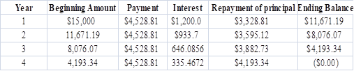
Table (20)
Steps required to calculate present value by using “PMT” function in excel are given,
- Select ‘Formulas’ option from Menu Bar of Excel sheet.
- Select insert Function that is (fx).
- Choose category of Financial.
- Then select “PMT” and then press OK.
- A window will pop up.
- Input data in the required field.
Amortization schedule represents annual payments, interest payments, principal payments, and beginning and ending loan balances.
Want to see more full solutions like this?
Chapter 5 Solutions
LMS Integrated for MindTap Finance, 1 term (6 months) Printed Access Card for Brigham/Houston's Fundamentals of Financial Management, Concise Edition, 9th

- Answer correctly otherwise unhelpfularrow_forwardYou've collected the following information from your favorite financial website. 52-Week Price Dividend Hi 77.40 Lo Stock (Dividend) Yield % PE Ratio Close Price Net Change 10.43 Acevedo .36 2.6 6 13.90 -.24 55.81 33.42 Georgette, Incorporated 1.54 3.8 10 40.43 -.01 131.04 70.05 YBM 2.55 2.9 10 89.08 3.07 50.24 35.00 13.95 Manta Energy .80 5.2 6 20.74 Winter Sports .32 1.5 28 15.43 ?? -.26 .18 According to analysts, the growth rate in dividends for YBM for the next five years is expected to be 21 percent. Suppose YBM meets this growth rate in dividends for the next five years and then the dividend growth rate falls to 5.75 percent, indefinitely. Assume investors require a return of 14 percent on YBM stock. According to the dividend growth model, what should the stock price be today? Note: Do not round intermediate calculations and round your answer to 2 decimal places, e.g., 32.16.)arrow_forward1. Waterfront Inc. wishes to borrow on a short-term basis without reducing its current ratio below 1.25. At present its current assets and current liabilities are $1,600 and $1,000 respectively. How much can Waterfront Inc. borrow?arrow_forward
- Question 3Footfall Manufacturing Ltd. reports the following financialinformation at the end of the current year:Net Sales $100,000Debtor’s turnover ratio (based onnet sales)2Inventory turnover ratio 1.25Fixed assets turnover ratio 0.8Debt to assets ratio 0.6Net profit margin 5%Gross profit margin 25%Return on investment 2%Use the given information to fill out the templates for incomestatement and balance sheet given below:Income Statement of Footfall Manufacturing Ltd. for the year endingDecember 31, 20XX(in $)Sales 100,000Cost of goodssoldGross profitOther expensesEarnings beforetaxTax @50%Earnings aftertaxBalance Sheet of Footfall Manufacturing Ltd. as at December 31, 20XX(in $)Liabilities Amount Assets AmountEquity Net fixed assetsLong termdebt50,000 InventoryShort termdebtDebtorsCashTOTAL TOTALarrow_forwardSolve correctly and no aiarrow_forwardSolvearrow_forward
- don't use chatgptIf data is unclear or blurr then comment i will write it.arrow_forwardIf data is unclear or blurr then comment i will write it. please don't use AI i will unhelpfularrow_forwardYou are considering an option to purchase or rent a single residential property. You can rent it for $5,000 per month and the owner would be responsible for maintenance, property insurance, and property taxes. Alternatively, you can purchase this property for $204,500 and finance it with an 80 percent mortgage loan at 4 percent interest that will fully amortize over a 30-year period. The loan can be prepaid at any time with no penalty. You have done research in the market area and found that (1) properties have historically appreciated at an annual rate of 2 percent per year, and rents on similar properties have also increased at 2 percent annually; (2) maintenance and insurance are currently $1,545.00 each per year and they have been increasing at a rate of 3 percent per year; (3) you are in a 24 percent marginal tax rate and plan to occupy the property as your principal residence for at least four years; (4) the capital gains exclusion would apply when you sell the property; (5)…arrow_forward
 Essentials Of InvestmentsFinanceISBN:9781260013924Author:Bodie, Zvi, Kane, Alex, MARCUS, Alan J.Publisher:Mcgraw-hill Education,

 Foundations Of FinanceFinanceISBN:9780134897264Author:KEOWN, Arthur J., Martin, John D., PETTY, J. WilliamPublisher:Pearson,
 Fundamentals of Financial Management (MindTap Cou...FinanceISBN:9781337395250Author:Eugene F. Brigham, Joel F. HoustonPublisher:Cengage Learning
 Corporate Finance (The Mcgraw-hill/Irwin Series i...FinanceISBN:9780077861759Author:Stephen A. Ross Franco Modigliani Professor of Financial Economics Professor, Randolph W Westerfield Robert R. Dockson Deans Chair in Bus. Admin., Jeffrey Jaffe, Bradford D Jordan ProfessorPublisher:McGraw-Hill Education