a.
To calculate: Future value of $1,000 after 5 years at 10% annual interest rate.
Introduction:
a.
Explanation of Solution
Calculation in spreadsheet by “FV” formula,
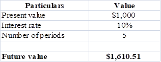
Table (1)
Steps required to calculate present value by using “FV” function in excel are given,
- Select ‘Formulas’ option from Menu Bar of Excel sheet.
- Select insert Function that is (fx).
- Choose category of Financial.
- Then select “FV” and then press OK.
- A window will pop up.
- Input data in the required field.
- Final answer will be shown by the formula that is $1,610.50.
Future value of $1,000 is $1,610.51.
b.
To calculate: Investments future value at 0%,5% and 20% rate after 0,1,2,3,4 and 5 years.
Introduction:
Time Value of Money: It is a vital concept to the investors, as it suggests them the money they are having today is worth more than the value promised in the future.
b.
Explanation of Solution
Calculation spreadsheet by “FV” formula,
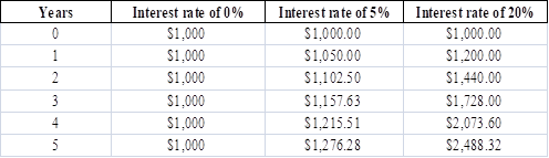
Table (2)
Steps required to calculate present value by using “FV” function in excel are given,
- Select ‘Formulas’ option from Menu Bar of Excel sheet.
- Select insert Function that is (fx).
- Choose category of Financial.
- Then select “FV” and then press OK.
- A window will pop up.
- Input data in required field.
Investment future values are different for the different years with 0%, 5% and 20% interest rate.
c.
To calculate: Present value due of $1,000 in 5 years at the discount rate of 10%.
Introduction:
Time Value of Money: It is a vital concept to the investors, as it suggests them the money they are having today is worth more than the value promised in the future.
c.
Explanation of Solution
Calculation in spreadsheet by “PV” formula,
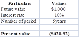
Table (3)
Steps required to calculate present value by using “PV” function in excel are given,
- Select ‘Formulas’ option from Menu Bar of Excel sheet.
- Select insert Function that is (fx).
- Choose category of Financial.
- Then select “PV” and then press OK.
- A window will pop up.
- Input data in the required field.
- Final answer will be shown by the formula that is $620.92.
Present value of $1,000 is $620.92 at 10 % discount rate.
d.
To calculate:
Introduction:
Time Value of Money: It is a vital concept to the investors, as it suggests them the money they are having today is worth more than the value promised in the future.
d.
Explanation of Solution
Calculationin spreadsheet by “RATE” formula,
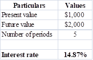
Table (4)
Steps required to calculate present value by using “RATE” function in excel are given,
- Select ‘Formulas’ option from Menu Bar of Excel sheet.
- Select insert Function that is (fx).
- Choose category of Financial.
- Then select “RATE” and then press OK.
- A window will pop up.
- Input data in the required field.
- Final answer will be shown by the formula that is 14.87%
The rate of return is14.87%.
e.
To calculate: Time taken by 36.5 million populations to double with annual growth rate of 2%
Introduction:
Time Value of Money: It is a vital concept to the investors, as it suggests them the money they are having today is worth more than the value promised in the future.
e.
Explanation of Solution
Calculation is solved in spreadsheet by “NPER” formula
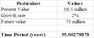
Table (5)
Steps required to calculate present value by using “NPER” function in excel are given,
- Select ‘Formulas’ option from Menu Bar of excel sheet.
- Select insert Function that is (fx).
- Choose category of Financial.
- Then select “NPER” and then press OK.
- A window will pop up.
- Input data in the required field.
- Final answer will be shown by the formula that is 35 years.
Conclusion:
It will take 35 years to double the population from 36.5 million to 73 million.
f.
To calculate: Present and future value of
Introduction:
Time Value of Money: It is a vital concept to the investors, as it suggests them the money they are having today is worth more than the value promised in the future.
f.
Explanation of Solution
Calculation in spreadsheet by “PV” formula,
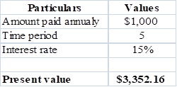
Table (6)
Steps required to calculate present value by using “PV” function in excel are given,
- Select ‘Formulas’ option from Menu Bar of Excel sheet.
- Select insert Function that is (fx).
- Choose category of Financial.
- Then select “PV” and then press OK.
- A window will pop up.
- Input data in the required field.
- Final answer will be shown by the formula that is $3,352.16.
So, the present value is $3,352.16.
Calculation of future value of
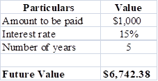
Table (7)
Steps required to calculate present value by using “FV” function in excel are given,
- Select ‘Formulas’ option from Menu Bar of Excel sheet.
- Select insert Function that is (fx).
- Choose category of Financial.
- Then select “FV” and then press OK.
- A window will pop up.
- Input data in the required field.
- Final answer will be shown by the formula that is $6,742.38.
So the future value is $6,742.38.
Present value is $3,352.16 and future value is $6,742.38 of
g.
To calculate: Present and future value of part ‘f’ if the
Introduction:
Time Value of Money: It is a vital concept to the investors, as it suggests them the money they are having today is worth more than the value promised in the future.
g.
Explanation of Solution
Calculation in spreadsheet by “PV” function,
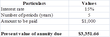
Table (8)
Steps required to calculate present value by using “PV” function in excel are given,
- Select ‘Formulas’ option from Menu Bar of Excel sheet.
- Select insert Function that is (fx).
- Choose category of Financial.
- Then select “PV” and then press OK.
- A window will pop up.
- Input data in the required field.
- Final answer will be shown by the formula that is $3,351.66.
Present value of
Future value of annuity in spreadsheet by “FV” function,
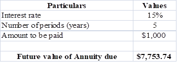
Table (9)
Steps required to calculate present value by using “FV” function in excel are given,
- Select ‘Formulas’ option from Menu Bar of Excel sheet.
- Select insert Function that is (fx).
- Choose category of Financial.
- Then select “FV” and then press OK.
- A window will pop up.
- Input data in the required field.
- Final answer will be shown by the formula that is $7,753.74
Future value of annuity due is $7,753.74.
Present value of
h.
To calculate: Present and future value for $1,000, due in 5 years with 10% semiannual compounding.
Introduction:
Time Value of Money: It is a vital concept to the investors, as it suggests them the money they are having today is worth more than the value promised in the future.
h.
Explanation of Solution
Calculation in spreadsheet by “PV” formula,
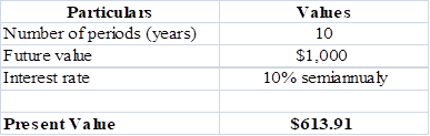
Table (10)
Steps required to calculate present value by using “PV” function in excel are given,
- Select ‘Formulas’ option from Menu Bar of Excel sheet.
- Select insert Function that is (fx).
- Choose category of Financial.
- Then select “PV” and then press OK.
- A window will pop up.
- Input data in the required field.
- Final answer will be shown by the formula that is $613.91.
Present value is $613.91.
Calculation in spreadsheet by “FV” formula,
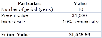
Table (11)
Steps required to calculate present value by using “FV” function in excel are given,
- Select ‘Formulas’ option from Menu Bar of Excel sheet.
- Select insert Function that is (fx).
- Choose category of Financial.
- Then select “FV” and then press OK.
- A window will pop up.
- Input data in the required field.
- Final answer will be shown by the formula that is $1,628.89.
Future value of
Present andfuture value for $1,000, due in 5 years with 10% semiannual compoundingwill be $613.91 and $1,628.89, respectively.
i.
To calculate: Annual payments for an ordinary
Introduction:
Time Value of Money: It is a vital concept to the investors, as it suggests them the money they are having today is worth more than the value promised in the future.
i.
Explanation of Solution
Calculation in spreadsheet by “PMT” formula,
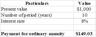
Table (12)
Steps required to calculate present value by using “PMT” function in excel are given,
- Select ‘Formulas’ option from Menu Bar of Excel sheet.
- Select insert Function that is (fx).
- Choose category of Financial.
- Then select “PMT” and then press OK.
- A window will pop up.
- Input data in the required field.
- Final answer will be shown by the formula that is $1,628.89.
Payment of ordinary
Calculation in spreadsheet by “PMT” formula,
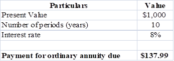
Table (13)
Steps required to calculate present value by using “PMT” function in excel are given,
- Select ‘Formulas’ option from Menu Bar of Excel sheet.
- Select insert Function that is (fx).
- Choose category of Financial.
- Then select “PMT” and then press OK.
- A window will pop up.
- Input data in the required field.
- Final answer will be shown by the formula that is $1,628.89.
Payment of ordinary annuity due is $137.99.
Annual payments are$149.03 for an ordinary
j.
To calculate: Present value and future value of an investment that pays 8% annually and makes the year end payments of $100, $200,$300.
j.
Explanation of Solution
Calculation in spreadsheet by “
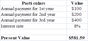
Table (14)
Steps required to calculate present value by using “NPV” function in excel are given,
- Select ‘Formulas’ option from Menu Bar of Excel sheet.
- Select insert Function that is (fx).
- Choose category of Financial.
- Then select “NPV” and then press OK.
- A window will pop up.
- Input data in the required field.
- Final answer will be shown by the formula that is $581.59.
Present value is $581.59.
Calculation in spreadsheet by “FV” formula,
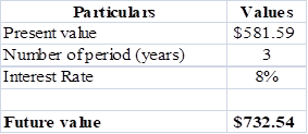
Table (15)
Steps required to calculate present value by using “FV” function in excel are given,
- Select ‘Formulas’ option from Menu Bar of Excel sheet.
- Select insert Function that is (fx).
- Choose category of Financial.
- Then select “FV” and then press OK.
- A window will pop up.
- Input data in the required field.
- Final answer will be shown by the formula that is $732.54.
Future value is $732.54.
Present value is $581.89 while future value is $732.54.
k.1.
To calculate: Effective annual rate each bank pays and the future value of $5,000 at the end of 1 and 2 year.
k.1.
Explanation of Solution
Given for Bank A,
Nominal interest rate is 5%.
Compounding is annual.
Formula to calculate effective annual rate is,
Where,
- EFF is the effective annual rate.
- INOM is the nominal interest rate.
- M is the compounding period.
Substitute 5% for INOM and 1 for M.
So, effective annual rate for Bank A is 5%.
Given for Bank B,
Nominal interest rate is 5%.
Compounding is semiannual.
Formula to calculate effective annual rate is,
Where,
- EFF is the effective annual rate.
- INOM is the nominal interest rate.
- M is the compounding period.
Substitute 5% for INOM and 2 for M.
So,effective annual rate for Bank B is 5.06%.
Given for Bank C,
Nominal interest rate is 5%.
Compounding is quarterly.
Formula to calculate effective annual rate is,
Where,
- EFF is the effective annual rate.
- INOM is the nominal interest rate.
- M is the compounding period.
Substitute 5% for INOM and 4 for M.
So, effective annual rate for Bank C is 5.09%.
Given for Bank D,
Nominal interest rate is 5%.
Compounding ismonthly.
Formula to calculate effective annual rate is,
Where,
- EFF is the effective annual rate.
- INOM is the nominal interest rate.
- M is the compounding period.
Substitute 5% for INOM and 12 for M.
So, effective annual rate for Bank D is 5.11%.
Given for Bank E,
Nominal interest rate is 5%.
Compounding is daily.
Formula to calculate effective annual rate is,
Where,
- EFF is the effective annual rate.
- INOM is the nominal interest rate.
- M is the compounding period.
Substitute 5% for INOM and 365 for M.
So, effective annual rate for Bank E is 5.12%.
Calculation of future value in spreadsheet by “FV” formula,
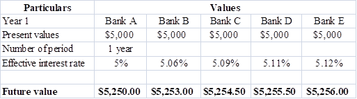
Table (16)
Steps required to calculate present value by using “FV” function in excel are given,
- Select ‘Formulas’ option from Menu Bar of Excel sheet.
- Select insert Function that is (fx).
- Choose category of Financial.
- Then select “FV” and then press OK.
- A window will pop up.
- Input data in the required field.
So, the future value at different effective rate after a year are $5, 250, $5,253,$5,254.50, $5,255.50 and $5,256.
Calculation of future value in spreadsheet by “FV” formula,
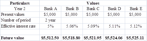
Table (17)
Steps required to calculate present value by using “FV” function in excel are given,
- Select ‘Formulas’ option from Menu Bar of Excel sheet.
- Select insert Function that is (fx).
- Choose category of Financial.
- Then select “FV” and then press OK.
- A window will pop up.
- Input data in the required field.
So, the future value at different effective rate after a year are $5, 512, $5,518.80, $5,521.95, $5,524.06 and $5,525.11.
Each bank pays different effective rate as there compounding is different, the rates are5% for bank A, 5.06% Bank B, 5.09% Bank C, 5.11% Bank D, 5.12% Bank E, also the future values also change on the basis of their number of periods.
2.
To explain: If banks are insured by the government and are equally risky, will they be equally able to attract funds and at what nominal rate all banks provide equal effective rate as Bank A.
2.
Answer to Problem 41SP
No, it is not possible for the banks to equally attract funds.
The nominal rate which causes same effective rate for all banks are,
| Particulars | A | B | C | D | E |
| Nominalrate | 5% | 5.06% | 5.09% | 5.11% | 5.12% |
Table (18)
Explanation of Solution
- Bank will not be equally able to attract funds because of compounding, as people prefer to invest in that bank which have more frequent compounding in comparison to the bank which have lesser frequent compounding.
- Nominal rate is opposite of the effective rate which is calculated in part ‘1’. The nominal rate indicated in above table will cause same effective rate for all banks as it is for A bank.
Due to frequent compounding, banks will not be able to equally attract funds and the nominal rate will be 5% for Bank A, 5.06% Bank B, 5.09% Bank C, 5.11% Bank D, 5.12% Bank E.
3.
To calculate: Present value of amount to get $5,000 after 1 year.
3.
Explanation of Solution
Calculation of payment to be made in spreadsheet by “PMT” formula,
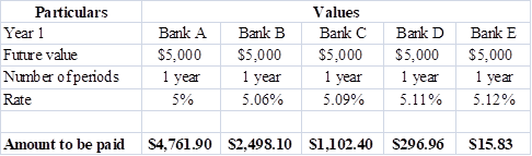
Table (19)
Steps required to calculate present value by using “PMT” function in excel are given,
- Select ‘Formulas’ option from Menu Bar of Excel sheet.
- Select insert Function that is (fx).
- Choose category of Financial.
- Then select “PMT” and then press OK.
- A window will pop up.
- Input data in the required field.
So, the amounts to be paid are$4,761.90,$2498.10,$1,102.40,$296.96 and $15.83.
4.
To explain: If all banks are providing a same effective interest rate would rational investor be indifferent between the banks.
4.
Answer to Problem 41SP
Yes, a rational investor would be indifferent between the banks.
Explanation of Solution
Rational investor chooses the bank which will provide him better return so he would be indifferent, if all the banks are giving same effective rate because he chooses the bank which will have more frequent compounding than others.
A bank offers frequent compounding is able to attract more number of customers than others.
To prepare: Amortization schedule to show annual payments, interest payments, principal payments, and beginning and ending loan balances.
Amortization:
Amotization means to write off or pay the debt over the priod of time it can be for loan or intangible assets. Its main purpose is to get cost recovery. Example of amortization is ,an automobile company that spent $20 million dollars on a design patent with a useful life of 20 years. The amortization value for that company will be $1 million each year.
Explanation of Solution
Calculation of annual installment is done by using “PMT” formula in spreadsheet at the amortization schedule.
Amortization schedule is prepared below,
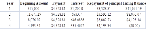
Table (20)
Steps required to calculate present value by using “PMT” function in excel are given,
- Select ‘Formulas’ option from Menu Bar of Excel sheet.
- Select insert Function that is (fx).
- Choose category of Financial.
- Then select “PMT” and then press OK.
- A window will pop up.
- Input data in the required field.
Amortization schedule represents annual payments, interest payments, principal payments, and beginning and ending loan balances.
Want to see more full solutions like this?
Chapter 5 Solutions
Fundamentals of Financial Management, Concise Edition (MindTap Course List)

- Assume that the following statements of financial position are stated and a book value. Alpha Corporation Current Assets $15,000 Current Liabilities $5,400 Net Fixed Assets 39,000 Long-Term Debt 10,100 Equity 38,500 $54,000 $54,000 Beta Corporation Current Assets $3,600 Current Liabilities $1,400 Net Fixed Assets 6,700 Long-Term Debt 2,100 Equity 6,800 $10,300 $10,300 Suppose the fair market value of Beta’s fixed assets is $9,500 rather than the $6,700 book value shown. Alpha pays $17,300 for Beta and raises the needed funds through an issue of long-term debt. Construct the post-merger statement of financial position now, assuming that the purchase method of accounting is used.arrow_forwardThe shareholders of Barley Corporation have voted in favor of a buyout offer from Wheat Corporation. Information about each firm is given here: Barley Wheat Price/earnings ratio 13.5 21 Shares outstanding 90,000 210,000 Earnings $180,000 $810,000 Barley shareholders will receive one share of Wheat stock for every three shares they hold of Barley. Required What will the EPS of Wheat be after the merger? What will be the P/E ratio if the NPV of the acquisition is 0? What must Wheat feel is the value of the synergy between these two firms? Explain how your answer can be reconciled with the decision to go ahead with the takeover?arrow_forwardBlack Oil Company is trying to decide whether to lease or buy a new computer-assisted drilling system for its extraction business. Management has already determined that acquisition of the system has a positive NPV. The system costs $9.4 million and qualifies for a 25% CCA rate. The equipment will have a $975,000 salvage value in five years. Black Oil’s tax rate is 36%, and the firm can borrow at 9%. Cape Town Company has offered to lease the drilling equipment to Black Oil for payments of $2.15 million per year. Cape Town’s policy is to require its lessees to make payments at the start of the year. Suppose it is estimated that the equipment will have no savage value at the end of the lease. What is the maximum lease payment acceptable to Black Oil now?arrow_forward
- Space Exploration Technology Corporation (Space X), is an aerospace manufacturer that sells stock engine components and tests equipment for commercial space transportation. A new customer has placed an order for eight high-bypass turbine engines, which increase fuel economy. The variable cost is $1.6 million per unit, and the credit price is $1.725 million each. Credit is extended for one period, and based on historical experience, payment for about one out of every 200 such orders is never collected. The required return is 1.8% per period. Required Assuming that this is a one-time order, should it be filled? The customer will not buy if credit is not extended. What is the break-even probability of default in part 1? Suppose that customers who don’t default become repeat customers and place the same order every period forever. Further assume that repeat customers never default. Should the order be filled? What is the break-even probability of default?arrow_forwardSouth African Airlines is contemplating leasing a high-tech tracker for its fleet of airplanes. Leasing is a very common practice with expensive, high-tech equipment. The scanner costs $6.3 million and it qualifies for a 30% CCA rate. Because of the rapid progression of technology, the high-tech tracker will be valued at $0 in 4 years. You can lease it for $1.875 million per year for four years. Assume that assets pool remains open and payments are made at the end of the year. Assuming a tax rate of 37%. You can borrow at 8% pre-tax. Should you lease or buy?arrow_forwardBlack Oil Company is trying to decide whether to lease or buy a new computer-assisted drilling system for its extraction business. Management has already determined that acquisition of the system has a positive NPV. The system costs $9.4 million and qualifies for a 25% CCA rate. The equipment will have a $975,000 salvage value in five years. Black Oil’s tax rate is 36%, and the firm can borrow at 9%. Cape Town Company has offered to lease the drilling equipment to Black Oil for payments of $2.15 million per year. Cape Town’s policy is to require its lessees to make payments at the start of the year. What is the NAL for Black Oil Company? What is the maximum lease payment that would be acceptable to the company?arrow_forward
- Iceberg Corporation currently has an all-equity capital structure. The company is considering a new structure that holds 30% debt. There are 6,500 shares outstanding and the price per share is $45 today. EBIT is expected to remain at $29,000 per year forever. The interest rate on new debt is 8%, and there are no taxes. Required Justin, a shareholder of the firm, owns 100 shares of stock. What is his cash flow under the current capital structure, assuming the company has a dividend payout rate of 100%? What will Justin’s cash flow be under the proposed capital structure of the firm? Assume he keeps all 100 of his shares. Suppose the company does convert, but Justin prefers the current all-equity capital structure. Show how he could unlever his shares of stock to recreate the original capital structure.arrow_forwardCovehead Lighthouse Corporation is considering a change in its cash-only policy. The new terms would be net one period. Based on the following information, determine if Covehead Lighthouse should proceed or not. The required rate of return is 2.5% per period. Current Policy New Policy Price per unit $73 $75 Cost per unit $38 $38 Unit sales per month 3,280 3,390arrow_forwardThe YYY and ZZZ Company are two firms whose business risk are the same but that have different dividend policies. YYY pays no dividend, whereas ZZZ has an expected dividend yield of 4%. Suppose the capital gains tax rate is zero, whereas the income tax rate is 35%. YYY has an expected earnings growth rate of 15% annually, and its stock price is expected to grow at this same rate. If the after-tax expected returns on the two stocks are equal, what is the pre-tax required return on ZZZ stock?arrow_forward
- Charlie Corporation is analyzing the possible acquisition of Delta Inc. Neither firm has debt. The forecasts of Charlie show that the purchase would increase its annual after-tax cash flow by $425,000 indefinitely. The current market value of Delta is $8.8 million. The current market value of Charlie is $22 million. The appropriate discount rate for the incremental cash flows is 8%. Charlie is trying to decide whether it should offer 35% of its stock or $12 million in cash to Delta. Required What is the synergy from the merger? What is the value of Delta to Charlie? What is the cost to Charlie of each alternative? What is the NPV of Charlie of each alternative?arrow_forwardParadox Corporation is evaluating an extra dividend verses a share repurchase. In either case, $14,500 would be spent. Current earnings are $1.65 per share, and the stock currently sells for $58 per share. There are 2,000 shares outstanding. Ignore taxes and other imperfections in answering the following questions: Required Evaluate the two alternatives in terms of the effect on the price per share of the stock and shareholder wealth. What will be the effect on Paradox Corporation’s EPS and P/E ratio under the two different scenarios? In the real world, which of these actions would you recommend? Why?arrow_forwardThe statement of financial position, from a market value, is shown below for AAA Corporation. AAA has declared a 25% stock dividend. The stock goes ex dividend tomorrow. There are currently 13,000 shares of stock outstanding. What will the ex-dividend price be? Market Value Statement of Financial Position Cash $83,000 Debt $121,000 Fixed Assets 575,000 Equity 537,000 Total $658,000 Total $658,000arrow_forward
 Essentials Of InvestmentsFinanceISBN:9781260013924Author:Bodie, Zvi, Kane, Alex, MARCUS, Alan J.Publisher:Mcgraw-hill Education,

 Foundations Of FinanceFinanceISBN:9780134897264Author:KEOWN, Arthur J., Martin, John D., PETTY, J. WilliamPublisher:Pearson,
 Fundamentals of Financial Management (MindTap Cou...FinanceISBN:9781337395250Author:Eugene F. Brigham, Joel F. HoustonPublisher:Cengage Learning
 Corporate Finance (The Mcgraw-hill/Irwin Series i...FinanceISBN:9780077861759Author:Stephen A. Ross Franco Modigliani Professor of Financial Economics Professor, Randolph W Westerfield Robert R. Dockson Deans Chair in Bus. Admin., Jeffrey Jaffe, Bradford D Jordan ProfessorPublisher:McGraw-Hill Education