
Concept explainers
Videos
One of the most surprising
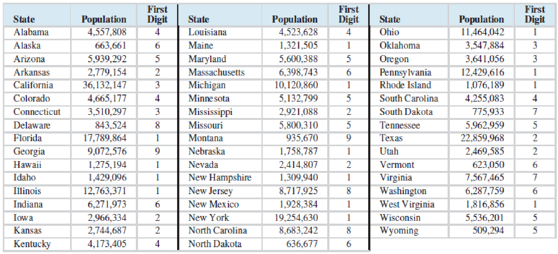
Following are the populations of the 50 states in a recent census. The first digit of each population number is listed separately.
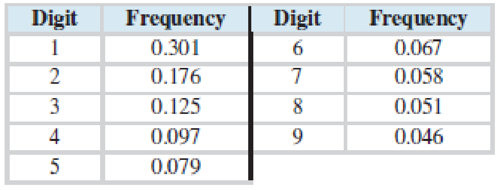
Here is a frequency distribution of the first digits of the state populations:
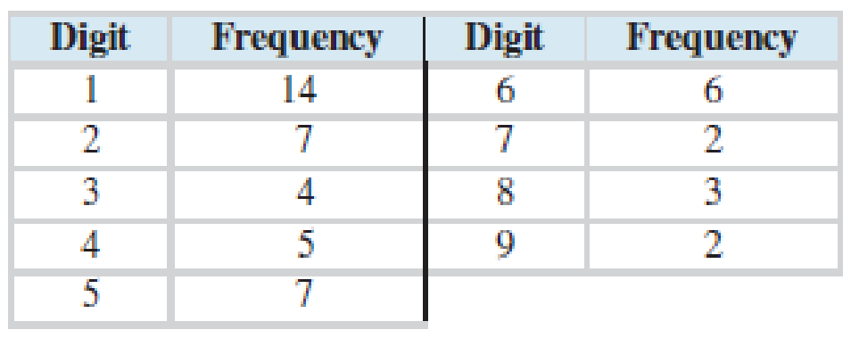
For the state populations, the most frequent first digit is 1, with 7, 8, and 9 being the least frequent.
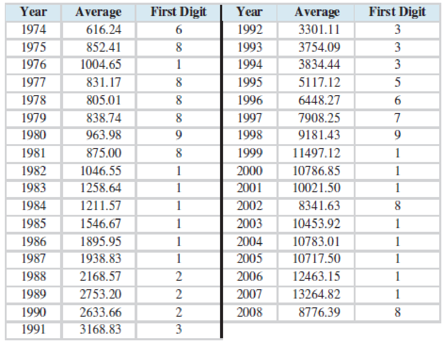
Now here is a table of the closing value of the Dow Jones Industrial Average for each of the years 1974–2008.
Here is a frequency distribution of the first digits of the stock market averages:
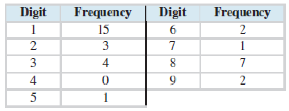
For the stock market averages, the most frequent first digit by far is 1.
The stock market averages give a partial justification for Benford’s law. Assume the stock market starts at 1000 and goes up 10% each year. It will take 8 years for the average to exceed 2000. Thus, the first eight averages will begin with the digit 1. Now imagine that the average starts at 5000. If it goes up 10% each year, it would take only 2 years to exceed 6000, so there would be only 2 years starting with the digit 5. In general, Benford’s law applies well to data where increments occur as a result of multiplication rather than addition, and where there is a wide
Here is the probability distribution of digits as predicted by Benford’s law:
The surprising nature of Benford’s law makes it a useful tool to detect fraud. When people make up numbers, they tend to make the first digits approximately uniformly distributed; in other words, they have approximately equal numbers of 1s, 2s, and so on. Many tax agencies, including the Internal Revenue Service, use software to detect deviations from Benford’s law in tax returns.
Following are results from three hypothetical corporate tax returns. Each purports to be a list of expenditures, in dollars, that the corporation is claiming as deductions. Two of the three are genuine, and one is a fraud. Which one is the fraud?
i. 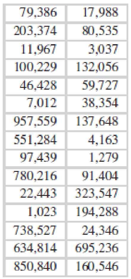
ii 
iii 
Want to see the full answer?
Check out a sample textbook solution
Chapter 5 Solutions
Essential Statistics


- 2. Hypothesis Testing - Two Sample Means A nutritionist is investigating the effect of two different diet programs, A and B, on weight loss. Two independent samples of adults were randomly assigned to each diet for 12 weeks. The weight losses (in kg) are normally distributed. Sample A: n = 35, 4.8, s = 1.2 Sample B: n=40, 4.3, 8 = 1.0 Questions: a) State the null and alternative hypotheses to test whether there is a significant difference in mean weight loss between the two diet programs. b) Perform a hypothesis test at the 5% significance level and interpret the result. c) Compute a 95% confidence interval for the difference in means and interpret it. d) Discuss assumptions of this test and explain how violations of these assumptions could impact the results.arrow_forward1. Sampling Distribution and the Central Limit Theorem A company produces batteries with a mean lifetime of 300 hours and a standard deviation of 50 hours. The lifetimes are not normally distributed—they are right-skewed due to some batteries lasting unusually long. Suppose a quality control analyst selects a random sample of 64 batteries from a large production batch. Questions: a) Explain whether the distribution of sample means will be approximately normal. Justify your answer using the Central Limit Theorem. b) Compute the mean and standard deviation of the sampling distribution of the sample mean. c) What is the probability that the sample mean lifetime of the 64 batteries exceeds 310 hours? d) Discuss how the sample size affects the shape and variability of the sampling distribution.arrow_forwardA biologist is investigating the effect of potential plant hormones by treating 20 stem segments. At the end of the observation period he computes the following length averages: Compound X = 1.18 Compound Y = 1.17 Based on these mean values he concludes that there are no treatment differences. 1) Are you satisfied with his conclusion? Why or why not? 2) If he asked you for help in analyzing these data, what statistical method would you suggest that he use to come to a meaningful conclusion about his data and why? 3) Are there any other questions you would ask him regarding his experiment, data collection, and analysis methods?arrow_forward
- Businessarrow_forwardWhat is the solution and answer to question?arrow_forwardTo: [Boss's Name] From: Nathaniel D Sain Date: 4/5/2025 Subject: Decision Analysis for Business Scenario Introduction to the Business Scenario Our delivery services business has been experiencing steady growth, leading to an increased demand for faster and more efficient deliveries. To meet this demand, we must decide on the best strategy to expand our fleet. The three possible alternatives under consideration are purchasing new delivery vehicles, leasing vehicles, or partnering with third-party drivers. The decision must account for various external factors, including fuel price fluctuations, demand stability, and competition growth, which we categorize as the states of nature. Each alternative presents unique advantages and challenges, and our goal is to select the most viable option using a structured decision-making approach. Alternatives and States of Nature The three alternatives for fleet expansion were chosen based on their cost implications, operational efficiency, and…arrow_forward
- The following ordered data list shows the data speeds for cell phones used by a telephone company at an airport: A. Calculate the Measures of Central Tendency from the ungrouped data list. B. Group the data in an appropriate frequency table. C. Calculate the Measures of Central Tendency using the table in point B. 0.8 1.4 1.8 1.9 3.2 3.6 4.5 4.5 4.6 6.2 6.5 7.7 7.9 9.9 10.2 10.3 10.9 11.1 11.1 11.6 11.8 12.0 13.1 13.5 13.7 14.1 14.2 14.7 15.0 15.1 15.5 15.8 16.0 17.5 18.2 20.2 21.1 21.5 22.2 22.4 23.1 24.5 25.7 28.5 34.6 38.5 43.0 55.6 71.3 77.8arrow_forwardII Consider the following data matrix X: X1 X2 0.5 0.4 0.2 0.5 0.5 0.5 10.3 10 10.1 10.4 10.1 10.5 What will the resulting clusters be when using the k-Means method with k = 2. In your own words, explain why this result is indeed expected, i.e. why this clustering minimises the ESS map.arrow_forwardwhy the answer is 3 and 10?arrow_forward

 Holt Mcdougal Larson Pre-algebra: Student Edition...AlgebraISBN:9780547587776Author:HOLT MCDOUGALPublisher:HOLT MCDOUGAL