Videos
a.
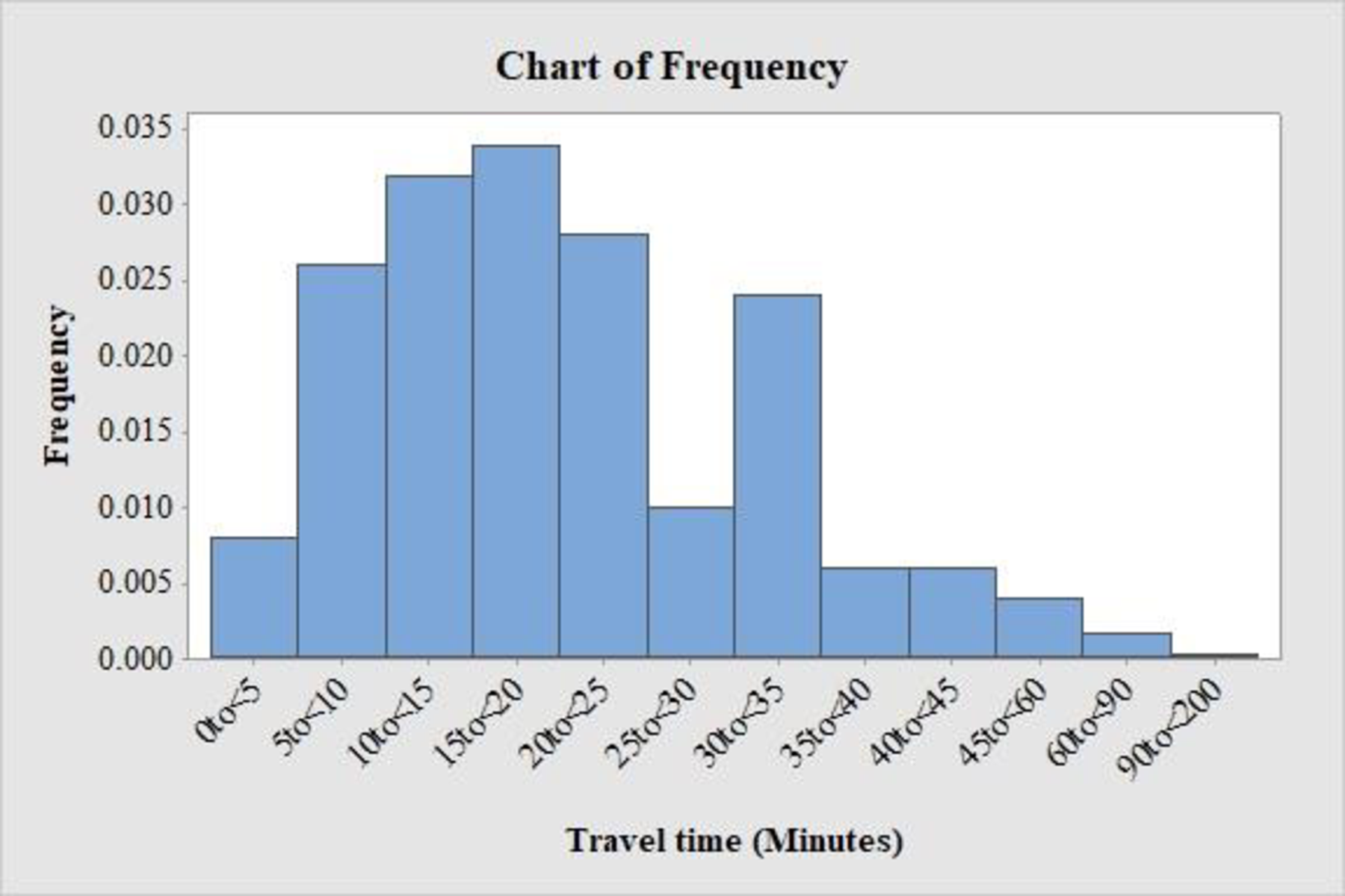
Draw a histogram for the travel time distribution.
a.
Answer to Problem 40E
The histogram for the travel time distribution is given below:
Explanation of Solution
Calculation:
The data represent the relative frequency for travel time to work for a large sample of adults who did not work at home.
Software procedure:
Step-by-step procedure to obtain the width using MINITAB software:
- Choose Calc > Calculator.
- Enter the column of width under Store result in variable.
- Enter the formula ‘Upper’-‘Lower’ under Expression.
- Click OK.
The
Step-by-step procedure to obtain the density using MINITAB software:
- Choose Calc > Calculator.
- Enter the column of Frequency under Store result in variable.
- Enter the formula ‘Frequency’/‘width’ under Expression.
- Click OK.
The density is stored in the column “Frequency”.
Step by step procedure to draw the relative frequency histogram using MINITAB software:
- Select Graph > Bar chart.
- In Bars represent select Values from a table.
- In One column of values select Simple.
- Enter Frequency in Graph variables.
- Enter Travel Time (Minutes) in categorical variable.
- Select OK.
- Click on the axis of the graph and in Gap between clusters enter 0.
Thus, the histogram for travel time is obtained.
b.
Delineate the features, such as center, shape, and variability of the histogram from Part (a).
b.
Explanation of Solution
From the histogram, it is observed that the distribution of travel time is slightly positively skewed with a single maximum frequency density, that is, a single
c.
Explain whether it is appropriate to use the
c.
Answer to Problem 40E
No, it is not appropriate to use empirical rule to make statements about the travel time distribution.
Explanation of Solution
By observing the histogram, the travel time data are skewed right. However, the empirical rule is applicable for data that are distributed normally, which is bell-shaped and symmetric.
Therefore, in this context, it is not appropriate to use the empirical rule to make the statements about the travel time distribution.
d.
Elucidate the reason why the travel time distribution could not be well approximated by a normal curve.
d.
Explanation of Solution
It is given that the approximate
The observation of the travel time should not be negative. In general, the travel time begins from 0.
If the distribution of the travel time is approximately normal, then the percentage of the travel time that fall below 0 is obtained as given below:
Use the standard normal probabilities (cumulative z-curve area) table to find the z-value:
Procedure:
For z at –1.12:
- Locate –1.1 in the left column of the table.
- Obtain the value in the corresponding row below 0.02.
That is,
Therefore, the percentage of the travel time that fall below 0 is 13.14% that is not possible.
Hence, the distribution of the travel time cannot be approximated by the normal curve.
e.
Find the percentage of travel time between 0 and 75 minutes using Chebyshev’s rule.
Obtain the percentage of travel time between 0 and 47 minutes using Chebyshev’s rule.
e.
Answer to Problem 40E
The percentage of travel time between 0 and 75 minutes is at least 75%.
The percentage of travel time between 0 and 47 minutes is at least 21%.
Explanation of Solution
Calculation:
The approximate mean and standard deviation for the travel time distribution are 27 minutes and 24 minutes, respectively.
The values at 2 standard deviations away from the mean is obtained as follows:
The observation of the travel time should not be negative. Therefore, the travel time that begins at –21 minutes lies in 2 standard deviation below the mean that is not possible. Travel time 75 minutes lies 2 standard deviations above from the mean.
Chebyshev’s rule:
For any number k, where
The z-score gives the number of standard deviations that an observation of 75 minutes is away from the mean. Here, the z-scores for 0 minutes and 75 minutes are –2 and 2, respectively. Thus, these observations of time are 2 standard deviations from the mean that is
(i).
The percentage of travel time between 0 and 75 minutes is obtained as given below:
Use Chebyshev’s rule as follows:
In this context, at least 0.75 proportion of observations lie within 2 standard deviations of the mean.
Therefore, the percentage of travel time between 0 and 75 minutes is 75%.
(ii).
A travel time of 47 minutes is
A travel time of 0 minutes is
Since 1.125 is larger than 0.833, these observations of time are 1.125 standard deviations from the mean that is
The percentage of the travel times between 0 and 47 minutes is obtained as given below:
Use Chebyshev’s rule as follows:
Thus, the percentage of the travel time between 0 and 47 minutes is 21%.
f.
Explain the way why the statements in Part (e) agree with the actual percentage for the travel time distribution.
f.
Explanation of Solution
Calculation:
The actual percentage of travel time between 0 and 75 minutes is obtained as given below:
Therefore, the actual percentage of travel time between 0 and 75 minutes is approximately 95.5% and differs a lot from the percentage obtained using Chebyshev’s rule.
The actual percentage of travel times between 0 and 47 minutes is obtained as given below:
Therefore, the actual percentage of travel time between 0 and 47 minutes is approximately 90% and differs a lot from the percentage obtained using Chebyshev’s rule.
Want to see more full solutions like this?
Chapter 4 Solutions
Introduction to Statistics and Data Analysis


- 1. If a firm spends more on advertising, is it likely to increase sales? Data on annual sales (in $100,000s) and advertising expenditures (in $10,000s) were collected for 20 firms in order to estimate the model Sales = Po + B₁Advertising + ε. A portion of the regression results is shown in the accompanying table. Intercept Advertising Standard Coefficients Error t Stat p-value -7.42 1.46 -5.09 7.66E-05 0.42 0.05 8.70 7.26E-08 a. Interpret the estimated slope coefficient. b. What is the sample regression equation? C. Predict the sales for a firm that spends $500,000 annually on advertising.arrow_forwardCan you help me solve problem 38 with steps im stuck.arrow_forwardHow do the samples hold up to the efficiency test? What percentages of the samples pass or fail the test? What would be the likelihood of having the following specific number of efficiency test failures in the next 300 processors tested? 1 failures, 5 failures, 10 failures and 20 failures.arrow_forward
- The battery temperatures are a major concern for us. Can you analyze and describe the sample data? What are the average and median temperatures? How much variability is there in the temperatures? Is there anything that stands out? Our engineers’ assumption is that the temperature data is normally distributed. If that is the case, what would be the likelihood that the Safety Zone temperature will exceed 5.15 degrees? What is the probability that the Safety Zone temperature will be less than 4.65 degrees? What is the actual percentage of samples that exceed 5.25 degrees or are less than 4.75 degrees? Is the manufacturing process producing units with stable Safety Zone temperatures? Can you check if there are any apparent changes in the temperature pattern? Are there any outliers? A closer look at the Z-scores should help you in this regard.arrow_forwardNeed help pleasearrow_forwardPlease conduct a step by step of these statistical tests on separate sheets of Microsoft Excel. If the calculations in Microsoft Excel are incorrect, the null and alternative hypotheses, as well as the conclusions drawn from them, will be meaningless and will not receive any points. 4. One-Way ANOVA: Analyze the customer satisfaction scores across four different product categories to determine if there is a significant difference in means. (Hints: The null can be about maintaining status-quo or no difference among groups) H0 = H1=arrow_forward
- Please conduct a step by step of these statistical tests on separate sheets of Microsoft Excel. If the calculations in Microsoft Excel are incorrect, the null and alternative hypotheses, as well as the conclusions drawn from them, will be meaningless and will not receive any points 2. Two-Sample T-Test: Compare the average sales revenue of two different regions to determine if there is a significant difference. (Hints: The null can be about maintaining status-quo or no difference among groups; if alternative hypothesis is non-directional use the two-tailed p-value from excel file to make a decision about rejecting or not rejecting null) H0 = H1=arrow_forwardPlease conduct a step by step of these statistical tests on separate sheets of Microsoft Excel. If the calculations in Microsoft Excel are incorrect, the null and alternative hypotheses, as well as the conclusions drawn from them, will be meaningless and will not receive any points 3. Paired T-Test: A company implemented a training program to improve employee performance. To evaluate the effectiveness of the program, the company recorded the test scores of 25 employees before and after the training. Determine if the training program is effective in terms of scores of participants before and after the training. (Hints: The null can be about maintaining status-quo or no difference among groups; if alternative hypothesis is non-directional, use the two-tailed p-value from excel file to make a decision about rejecting or not rejecting the null) H0 = H1= Conclusion:arrow_forwardPlease conduct a step by step of these statistical tests on separate sheets of Microsoft Excel. If the calculations in Microsoft Excel are incorrect, the null and alternative hypotheses, as well as the conclusions drawn from them, will be meaningless and will not receive any points. The data for the following questions is provided in Microsoft Excel file on 4 separate sheets. Please conduct these statistical tests on separate sheets of Microsoft Excel. If the calculations in Microsoft Excel are incorrect, the null and alternative hypotheses, as well as the conclusions drawn from them, will be meaningless and will not receive any points. 1. One Sample T-Test: Determine whether the average satisfaction rating of customers for a product is significantly different from a hypothetical mean of 75. (Hints: The null can be about maintaining status-quo or no difference; If your alternative hypothesis is non-directional (e.g., μ≠75), you should use the two-tailed p-value from excel file to…arrow_forward
- Please conduct a step by step of these statistical tests on separate sheets of Microsoft Excel. If the calculations in Microsoft Excel are incorrect, the null and alternative hypotheses, as well as the conclusions drawn from them, will be meaningless and will not receive any points. 1. One Sample T-Test: Determine whether the average satisfaction rating of customers for a product is significantly different from a hypothetical mean of 75. (Hints: The null can be about maintaining status-quo or no difference; If your alternative hypothesis is non-directional (e.g., μ≠75), you should use the two-tailed p-value from excel file to make a decision about rejecting or not rejecting null. If alternative is directional (e.g., μ < 75), you should use the lower-tailed p-value. For alternative hypothesis μ > 75, you should use the upper-tailed p-value.) H0 = H1= Conclusion: The p value from one sample t-test is _______. Since the two-tailed p-value is _______ 2. Two-Sample T-Test:…arrow_forwardPlease conduct a step by step of these statistical tests on separate sheets of Microsoft Excel. If the calculations in Microsoft Excel are incorrect, the null and alternative hypotheses, as well as the conclusions drawn from them, will be meaningless and will not receive any points. What is one sample T-test? Give an example of business application of this test? What is Two-Sample T-Test. Give an example of business application of this test? .What is paired T-test. Give an example of business application of this test? What is one way ANOVA test. Give an example of business application of this test? 1. One Sample T-Test: Determine whether the average satisfaction rating of customers for a product is significantly different from a hypothetical mean of 75. (Hints: The null can be about maintaining status-quo or no difference; If your alternative hypothesis is non-directional (e.g., μ≠75), you should use the two-tailed p-value from excel file to make a decision about rejecting or not…arrow_forwardThe data for the following questions is provided in Microsoft Excel file on 4 separate sheets. Please conduct a step by step of these statistical tests on separate sheets of Microsoft Excel. If the calculations in Microsoft Excel are incorrect, the null and alternative hypotheses, as well as the conclusions drawn from them, will be meaningless and will not receive any points. What is one sample T-test? Give an example of business application of this test? What is Two-Sample T-Test. Give an example of business application of this test? .What is paired T-test. Give an example of business application of this test? What is one way ANOVA test. Give an example of business application of this test? 1. One Sample T-Test: Determine whether the average satisfaction rating of customers for a product is significantly different from a hypothetical mean of 75. (Hints: The null can be about maintaining status-quo or no difference; If your alternative hypothesis is non-directional (e.g., μ≠75), you…arrow_forward
 Big Ideas Math A Bridge To Success Algebra 1: Stu...AlgebraISBN:9781680331141Author:HOUGHTON MIFFLIN HARCOURTPublisher:Houghton Mifflin Harcourt
 Holt Mcdougal Larson Pre-algebra: Student Edition...AlgebraISBN:9780547587776Author:HOLT MCDOUGALPublisher:HOLT MCDOUGAL
 Functions and Change: A Modeling Approach to Coll...AlgebraISBN:9781337111348Author:Bruce Crauder, Benny Evans, Alan NoellPublisher:Cengage Learning
 Glencoe Algebra 1, Student Edition, 9780079039897...AlgebraISBN:9780079039897Author:CarterPublisher:McGraw Hill
 College Algebra (MindTap Course List)AlgebraISBN:9781305652231Author:R. David Gustafson, Jeff HughesPublisher:Cengage Learning
 Mathematics For Machine TechnologyAdvanced MathISBN:9781337798310Author:Peterson, John.Publisher:Cengage Learning,