Concept explainers
Videos
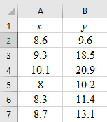
Incoine: Medicai Care Let x be per capita income in thousands of dollars. Let y be the number of medical doctors per 10,000 residents. Six small cities in Oregon gave the following information about x and y(based on information from Lifein America's Small Cities by G. S. Thomas, Prometheus Books).
| x | 8.6 | 9.3 | 10.1 | 8.0 | 8.3 | 8.7 |
| y | 9.6 | 18.5 | 20.9 | 10.2 | 11.4 | 13.1 |
Complete parts (a) through (e), given
(a)
To graph: The scatter diagram.
Explanation of Solution
Given: The data that consists of the variables ‘per capita income in thousands of dollars’ and ‘the number of medical doctors per 10,000 residents’, which are represented by x and y, respectively, are provided.
Graph:
Follow the steps given below in MS Excel to obtain the scatter diagram of the data.
Step 1: Enter the data into an MS Excel sheet. The screenshot is given below.
Step 2: Select the data and click on ‘Insert’. Go to ‘charts’ and select ‘Scatter’ as the chart type.
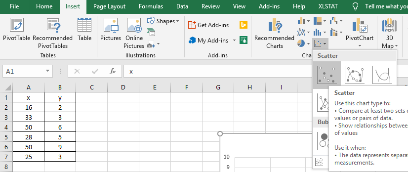
Step 3: Select the first plot and click the ‘add chart element’ option provided in the left-hand corner of the menu bar. Insert the ‘Axis titles’ and the ‘Chart title’. The scatter plot for the provided data is shown below.
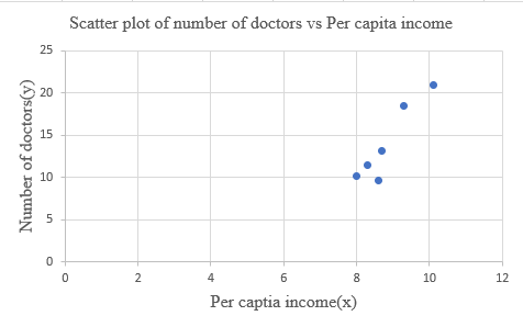
Interpretation: The scatterplot shows that the correlation between the per capita income (x) and the number of medical doctors (y) is positive. So, as x increases (or decreases), the value of y increases (or decreases).
(b)
To test: Whether the provided values of
Answer to Problem 13P
Solution: The provided values, that is,
Explanation of Solution
Given: The provided values are
Calculation:
To compute
| 8.6 | 9.6 | 73.96 | 92.16 | 82.56 |
| 9.3 | 18.5 | 86.49 | 342.25 | 172.05 |
| 10.1 | 20.9 | 102.01 | 436.81 | 211.09 |
| 8 | 10.2 | 64 | 104.04 | 81.6 |
| 8.3 | 11.4 | 68.89 | 129.96 | 94.62 |
| 8.7 | 13.1 | 75.69 | 171.61 | 113.97 |
Now, the value of
Substitute the values in the above formula. Thus:
Thus, the value of
Conclusion: The provided values, that is,
(c)
To find: The values of
Answer to Problem 13P
Solution: The calculated values are
Explanation of Solution
Given: The provided values are
Calculation:
The value of
The value of
The value of
The value of
Therefore, the values are
The general formula of a least-squares line is:
Here, a is the y-intercept and b is the slope.
Substitute the values of a and b in the general equation to get the equation of the least-squares line of the data as follows:
Therefore, the least-squares line equation is
(d)
To graph: The least-squares line on the scatter diagram that passes through the point
Explanation of Solution
Given: The data that consists of the variables ‘per capita income’ and ‘the number of medical doctors per 10,000 residents’, which are represented by x and y, respectively, are provided.
Graph:
Follow the steps given below in MS Excel to obtain the scatter diagram of the data.
Step 1: Enter the data into an MS Excel sheet. The screenshot is given below.
Step 2: Select the data and click on ‘Insert’. Go to ‘charts’ and select ‘Scatter’ as the chart type.
Step 3: Select the first plot and click the ‘add chart element’ option provided in the left-hand corner of the menu bar. Insert the ‘Axis titles’ and the ‘Chart title’. The scatter plot for the provided data is shown below.
Step 4: Right click on any data point and select ‘Add Trendline’. In the dialogue box, select ‘linear’ and check ‘Display Equation on Chart’. The scatter diagram with the least-squares line is given below.
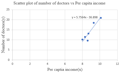
Interpretation: The least-squares line passes through the point
(e)
The value of
Answer to Problem 13P
Solution: The value of
Explanation of Solution
Given: The value of the correlation coefficient (r) is
Calculation: The coefficient of determination
Therefore, the value of
Further, the proportion of variation in y that cannot be explained can be calculated as:
Hence, the percentage of variation in y that cannot be explained is 12.8%.
Interpretation: About 87.2% of the variation in y can be explained by the corresponding variation in x and the least-squares line while the remaining 12.8% of variation cannot be explained.
(f)
To find: The predicted number of MDs (medical doctors) per 10,000 residents.
Answer to Problem 13P
Solution: The predicted value is 20.7 physicians per 10,000 residents.
Explanation of Solution
Given: The least-squares line from part (c) is
Calculation:
The predicted value
Thus, the value of
Interpretation: The predicted number of medical doctors per 10,000 residents for a city with a per capita income of 10 thousand dollars is 20.7.
Want to see more full solutions like this?
Chapter 4 Solutions
Understanding Basic Statistics


- please find the answers for the yellows boxes using the information and the picture belowarrow_forwardA marketing agency wants to determine whether different advertising platforms generate significantly different levels of customer engagement. The agency measures the average number of daily clicks on ads for three platforms: Social Media, Search Engines, and Email Campaigns. The agency collects data on daily clicks for each platform over a 10-day period and wants to test whether there is a statistically significant difference in the mean number of daily clicks among these platforms. Conduct ANOVA test. You can provide your answer by inserting a text box and the answer must include: also please provide a step by on getting the answers in excel Null hypothesis, Alternative hypothesis, Show answer (output table/summary table), and Conclusion based on the P value.arrow_forwardA company found that the daily sales revenue of its flagship product follows a normal distribution with a mean of $4500 and a standard deviation of $450. The company defines a "high-sales day" that is, any day with sales exceeding $4800. please provide a step by step on how to get the answers Q: What percentage of days can the company expect to have "high-sales days" or sales greater than $4800? Q: What is the sales revenue threshold for the bottom 10% of days? (please note that 10% refers to the probability/area under bell curve towards the lower tail of bell curve) Provide answers in the yellow cellsarrow_forward
- Business Discussarrow_forwardThe following data represent total ventilation measured in liters of air per minute per square meter of body area for two independent (and randomly chosen) samples. Analyze these data using the appropriate non-parametric hypothesis testarrow_forwardeach column represents before & after measurements on the same individual. Analyze with the appropriate non-parametric hypothesis test for a paired design.arrow_forward
 Algebra: Structure And Method, Book 1AlgebraISBN:9780395977224Author:Richard G. Brown, Mary P. Dolciani, Robert H. Sorgenfrey, William L. ColePublisher:McDougal Littell
 Glencoe Algebra 1, Student Edition, 9780079039897...AlgebraISBN:9780079039897Author:CarterPublisher:McGraw Hill
 Elementary Geometry For College Students, 7eGeometryISBN:9781337614085Author:Alexander, Daniel C.; Koeberlein, Geralyn M.Publisher:Cengage,
 College Algebra (MindTap Course List)AlgebraISBN:9781305652231Author:R. David Gustafson, Jeff HughesPublisher:Cengage Learning
 College AlgebraAlgebraISBN:9781305115545Author:James Stewart, Lothar Redlin, Saleem WatsonPublisher:Cengage Learning
 Mathematics For Machine TechnologyAdvanced MathISBN:9781337798310Author:Peterson, John.Publisher:Cengage Learning,