
Concept explainers
Videos
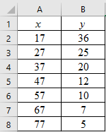
Auto Accidents: Age Data for this problem are based on information taken from The Wall Street Journal. Let x be the age in years of a licensed automobile driver. Let y be the percentage of all fatal accidents (for a given age) due to speeding. For example, the first data pair indicates that 36% of all fatal accidents involving 17-year-olds are due to speeding.
| x | 17 | 27 | 37 | 47 | 57 | 67 | 77 |
| y | 36 | 25 | 20 | 12 | 10 | 7 | 5 |
Complete parts (a) through (e), given
(f) Predict the percentage of all fatal accidents due to speeding for 25-year-olds.
(a)
To graph: The scatter diagram for age in years of a licensed automobile driver (x) and percentage of all fatal accidents (y).
Explanation of Solution
Given: The data which consists of variables, ‘age of a licensed automobile driver (in years)’ and ‘the percentage of all fatal accidents (for a given age)’ due to speeding, represented by x and y respectively, is provided.
Graph:
Follow the steps given below in Excel to obtain the scatter diagram of the data.
Step 1: Enter the data into Excel sheet. The screenshot is given below.
Step 2: Select the data and click on ‘Insert’. Go to charts and select the chart type ‘Scatter’.

Step 3: Select the first plot and then click ‘add chart element’ provided in the left corner of the menu bar. Insert the ‘Axis titles’ and ‘Chart title’. The scatter plot for the provided data is shown below:
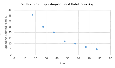
Interpretation: The scatterplot shows that, there is a negative correlation between the age of a licensed automobile drivers and the speeding- related fatal percentage. So, as the age increases, the fatal percentage related to speeding decreases and vice versa.
(b)
To test: Whether the provided values of
Answer to Problem 11P
Solution: The provided values, that is,
Explanation of Solution
Given: The provided values are:
Calculation:
To compute
| 17 | 36 | 289 | 1296 | 612 |
| 27 | 25 | 729 | 625 | 675 |
| 37 | 20 | 1369 | 400 | 740 |
| 47 | 12 | 2209 | 144 | 564 |
| 57 | 10 | 3249 | 100 | 570 |
| 67 | 7 | 4489 | 49 | 469 |
| 77 | 5 | 5929 | 25 | 385 |
Now, the value of
Substituting the values in the above formula. Thus:
Thus, the value of
Conclusion: The provided values,
(c)
To find: The values of
Answer to Problem 11P
Solution: The calculated values are,
Explanation of Solution
Given: The provided values are,
Calculation:
The value of
The value of
The value of
The value of
Therefore, the values are,
The general formula for the least-squares line is,
Here, a is the y-intercept and b is the slope.
Substitute the values of a and b in the general equation, to get the least-squares line of the data. That is,
Therefore, the least-squares line is
(d)
To graph: The least-squares line on the scatter diagram which passes through the point
Explanation of Solution
Given: The data which consists of variables, ‘age of a licensed automobile driver (in years)’ and ‘the fatal accidents percentage (for a given age) due to speeding’, represented by x and y respectively, is provided.
Graph:
Follow the steps given below in Excel to obtain the scatter diagram of the data.
Step 1: Enter the data into Excel sheet. The screenshot is given below.
Step 2: Select the data and click on ‘Insert’. Go to charts and select the chart type ‘Scatter’.
Step 3: Select the first plot and then click ‘add chart element’ provided in the left corner of the menu bar. Insert the ‘Axis titles’ and ‘Chart title’. The scatter plot for the provided data is shown below:
Step 3: Right click on any data point and select ‘Add Trendline’. In the dialogue box, select ‘linear’ and check ‘Display Equation on Chart’
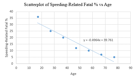
Interpretation: The least-squares line passes through the point
(e)
The value of
Answer to Problem 11P
Solution: The value of
Explanation of Solution
Given: The value of the correlation coefficient (r) is
Calculation: The coefficient of determination
Therefore, the value of
The value of
Further, the proportion of variation in y that is unexplained can be calculated as:
Hence, the percentage of variation in y that is unexplained is 8%.
Interpretation: About 92% of the variation in y (fatal % due to speeding) can be explained by the corresponding variation in x (age) and the least-squares line. The rest 8% of variation remains unexplained.
(f)
To find: The predicted percentage of speeding related fatal accidents
Answer to Problem 11P
Solution: The predicted value is approximately 27.36%.
Explanation of Solution
Given: The least-squares line from part (c) is,
Calculation:
The predicted value
Thus, the value of
Interpretation: The percentage of all fatal accidents due to speeding for 25-years-olds is predicted to be 27.36%.
Want to see more full solutions like this?
Chapter 4 Solutions
EBK UNDERSTANDING BASIC STATISTICS


- please find the answers for the yellows boxes using the information and the picture belowarrow_forwardA marketing agency wants to determine whether different advertising platforms generate significantly different levels of customer engagement. The agency measures the average number of daily clicks on ads for three platforms: Social Media, Search Engines, and Email Campaigns. The agency collects data on daily clicks for each platform over a 10-day period and wants to test whether there is a statistically significant difference in the mean number of daily clicks among these platforms. Conduct ANOVA test. You can provide your answer by inserting a text box and the answer must include: also please provide a step by on getting the answers in excel Null hypothesis, Alternative hypothesis, Show answer (output table/summary table), and Conclusion based on the P value.arrow_forwardA company found that the daily sales revenue of its flagship product follows a normal distribution with a mean of $4500 and a standard deviation of $450. The company defines a "high-sales day" that is, any day with sales exceeding $4800. please provide a step by step on how to get the answers Q: What percentage of days can the company expect to have "high-sales days" or sales greater than $4800? Q: What is the sales revenue threshold for the bottom 10% of days? (please note that 10% refers to the probability/area under bell curve towards the lower tail of bell curve) Provide answers in the yellow cellsarrow_forward
- Business Discussarrow_forwardThe following data represent total ventilation measured in liters of air per minute per square meter of body area for two independent (and randomly chosen) samples. Analyze these data using the appropriate non-parametric hypothesis testarrow_forwardeach column represents before & after measurements on the same individual. Analyze with the appropriate non-parametric hypothesis test for a paired design.arrow_forward
 Glencoe Algebra 1, Student Edition, 9780079039897...AlgebraISBN:9780079039897Author:CarterPublisher:McGraw Hill
 Functions and Change: A Modeling Approach to Coll...AlgebraISBN:9781337111348Author:Bruce Crauder, Benny Evans, Alan NoellPublisher:Cengage Learning
 Big Ideas Math A Bridge To Success Algebra 1: Stu...AlgebraISBN:9781680331141Author:HOUGHTON MIFFLIN HARCOURTPublisher:Houghton Mifflin Harcourt
 Holt Mcdougal Larson Pre-algebra: Student Edition...AlgebraISBN:9780547587776Author:HOLT MCDOUGALPublisher:HOLT MCDOUGAL
 Linear Algebra: A Modern IntroductionAlgebraISBN:9781285463247Author:David PoolePublisher:Cengage Learning