
Videos
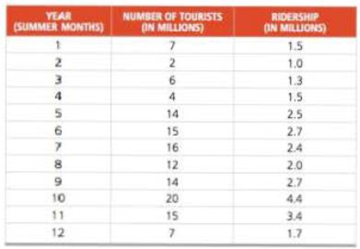
Bus and subway ridership for the summer months in London, England, is believed to be tied heavily to the number of tourists visiting the city. During the past 12 years, the data on the next page have been obtained:
a) Plot these data and decide if a linear model is reasonable.
b) Develop a regression relationship.
c) What is expected ridership if 10 million tourists visit London in a year?
d) Explain the predicted ridership if there are no tourists at all.
e) What is the standard error of the estimate?
f) What is the model’s correlation coefficient and coefficient of determination?
a)
To determine: To plot the data and decide whether the linear model is reasonable.
Introduction: Forecasting is used to predict future changes or demand patterns. It involves different approaches and varies with different periods.
Answer to Problem 52P
The graph for the given data is plotted and it can be observed that the data points are scattered around.
Explanation of Solution
Given information:
| Year (Summer Months) | Number of tourist (in millions) | Ridership (in millions) |
| 1 | 7 | 1.5 |
| 2 | 2 | 1 |
| 3 | 6 | 1.3 |
| 4 | 4 | 1.5 |
| 5 | 14 | 2.5 |
| 6 | 15 | 2.7 |
| 7 | 16 | 2.4 |
| 8 | 12 | 2 |
| 9 | 14 | 2.7 |
| 10 | 20 | 4.4 |
| 11 | 15 | 3.4 |
| 12 | 7 | 1.7 |
Table 1
Graphical representation:
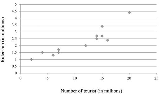
The data to plot the graph is taken from Table 1.
Hence, the graph for the given data is plotted and it can be observed that the data points are scattered around.
b)
To determine: A regression relationship.
Answer to Problem 52P
The linear regression equation is
Explanation of Solution
Given information:
| Year (Summer Months) | Number of tourist (in millions) | Ridership (in millions) |
| 1 | 7 | 1.5 |
| 2 | 2 | 1 |
| 3 | 6 | 1.3 |
| 4 | 4 | 1.5 |
| 5 | 14 | 2.5 |
| 6 | 15 | 2.7 |
| 7 | 16 | 2.4 |
| 8 | 12 | 2 |
| 9 | 14 | 2.7 |
| 10 | 20 | 4.4 |
| 11 | 15 | 3.4 |
| 12 | 7 | 1.7 |
Formula of least square regression:
Where,
Where,
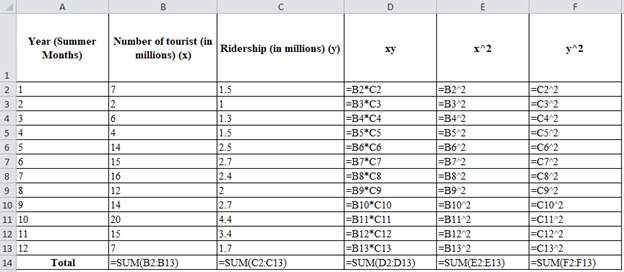
| Year (Summer Months) | Number of tourist (in millions) (x) | Ridership (in millions) (y) | xy | x^2 | y^2 |
| 1 | 7 | 1.5 | 10.5 | 49 | 2.25 |
| 2 | 2 | 1 | 2 | 4 | 1 |
| 3 | 6 | 1.3 | 7.8 | 36 | 1.69 |
| 4 | 4 | 1.5 | 6 | 16 | 2.25 |
| 5 | 14 | 2.5 | 35 | 196 | 6.25 |
| 6 | 15 | 2.7 | 40.5 | 225 | 7.29 |
| 7 | 16 | 2.4 | 38.4 | 256 | 5.76 |
| 8 | 12 | 2 | 24 | 144 | 4 |
| 9 | 14 | 2.7 | 37.8 | 196 | 7.29 |
| 10 | 20 | 4.4 | 88 | 400 | 19.36 |
| 11 | 15 | 3.4 | 51 | 225 | 11.56 |
| 12 | 7 | 1.7 | 11.9 | 49 | 2.89 |
| Total | 132 | 27.1 | 352.9 | 1796 | 71.59 |
Table 2
Excel worksheet:
Substitute the values in the above formula.
Calculation of the average of x values
The average of x values is obtained by dividing the summation of x values with the number of periods n=12, the value of
Calculation of the average of y values
The average of y values is obtained by dividing the summation of sales with the number of periods n=12. The value of
Calculation ofthe slope of regression line‘b’:
The summation of the product of sales (y) with x values is ∑xy = 352.9, the product of number of period (n), the average of x values and the average of y values is obtained;
The summation of the square of x values, 1796, is subtracted from the product of the number of periods, 10with the average of x values, 11. The resultant value is 344. The slope of the regression line is obtained by dividing 1796 with 344. The value of ‘b’ is 0.159.
Calculation of the y-axis intercept ‘a’:
The y-axis intercept is obtained by the difference between the average of y values and values obtained by the product of the slope of regression line with the average of x values. The resultant value of ‘a’ is 0.511.
Least Square Regression forecasting equation:
Substitute the slope of regression line and they axis intercept in the regression equation which gives the liner regression equation for the data.
Hence, the linear regression equation is
c)
To determine: The expected ridership when 10 million tourists visit in a year.
Answer to Problem 52P
There is a 2.101 million ridership when 10 million tourists visit in a year.
Explanation of Solution
Given information:
| Year (Summer Months) | Number of tourist (in millions) | Ridership (in millions) |
| 1 | 7 | 1.5 |
| 2 | 2 | 1 |
| 3 | 6 | 1.3 |
| 4 | 4 | 1.5 |
| 5 | 14 | 2.5 |
| 6 | 15 | 2.7 |
| 7 | 16 | 2.4 |
| 8 | 12 | 2 |
| 9 | 14 | 2.7 |
| 10 | 20 | 4.4 |
| 11 | 15 | 3.4 |
| 12 | 7 | 1.7 |
Formula of least square regression:
Where,
Where,
Calculation of number of ridership when 10 million touristsvisit in a year:
Equation (1) provides the linear regression equation for the data and substitutes the number of tourists visiting in the regression equation. Substituting 10 million in the equation, the resultant value is found to be 2.101 million ridership.
Hence, there are 2.101 million ridership when 10 million touristsvisit in a year.
d)
To determine: The expected ridership when no tourists visit in a year.
Answer to Problem 52P
There is a 511,000 ridership when no touristsvisit in a year.
Explanation of Solution
Given information:
| Year (Summer Months) | Number of tourist (in millions) | Ridership (in millions) |
| 1 | 7 | 1.5 |
| 2 | 2 | 1 |
| 3 | 6 | 1.3 |
| 4 | 4 | 1.5 |
| 5 | 14 | 2.5 |
| 6 | 15 | 2.7 |
| 7 | 16 | 2.4 |
| 8 | 12 | 2 |
| 9 | 14 | 2.7 |
| 10 | 20 | 4.4 |
| 11 | 15 | 3.4 |
| 12 | 7 | 1.7 |
Formula of least square regression:
Where,
Where,
Calculation of the number of ridership when notouristsvisit in a year:
Equation (1) provides the linear regression equation for the data and substitutes the number of tourists visiting in the regression equation. Substituting 0 in the equation, the resultant value is 0.511 million ridership.
Hence, there is a 511,000 ridership when notouristsvisit in a year.
e)
To determine: The standard error of estimate.
Answer to Problem 52P
The standard error of estimate is0.4037.
Explanation of Solution
Given information:
| Year (Summer Months) | Number of tourists(in millions) | Ridership (in millions) |
| 1 | 7 | 1.5 |
| 2 | 2 | 1 |
| 3 | 6 | 1.3 |
| 4 | 4 | 1.5 |
| 5 | 14 | 2.5 |
| 6 | 15 | 2.7 |
| 7 | 16 | 2.4 |
| 8 | 12 | 2 |
| 9 | 14 | 2.7 |
| 10 | 20 | 4.4 |
| 11 | 15 | 3.4 |
| 12 | 7 | 1.7 |
Formula to compute the standard error of estimate:
Calculation of standard error of estimate:
The values to be substituted in the standard error of estimate formula are given inTable 2. Substitute the values from the table in the formula. This results in a standard error of estimate of 0.4037.
Hence, the standard error of estimate is 0.4037.
f)
To determine: The coefficient of correlation (r) and coefficient of determination (r2).
Answer to Problem 52P
The coefficient of correlation (r) and coefficient of determination (r2) are 717.41 & 0.840, respectively.
Explanation of Solution
Given information:
| Year (Summer Months) | Number of tourists(in millions) | Ridership (in millions) |
| 1 | 7 | 1.5 |
| 2 | 2 | 1 |
| 3 | 6 | 1.3 |
| 4 | 4 | 1.5 |
| 5 | 14 | 2.5 |
| 6 | 15 | 2.7 |
| 7 | 16 | 2.4 |
| 8 | 12 | 2 |
| 9 | 14 | 2.7 |
| 10 | 20 | 4.4 |
| 11 | 15 | 3.4 |
| 12 | 7 | 1.7 |
Formula to calculate the correlation coefficient:
Calculation of the correlation coefficient (r):
Table (2) provides the values to calculate the correlation coefficient (r).
Calculation of the correlation of determination (r2):
Hence, the coefficient of correlation and coefficient of determination are 717.41 and 0.840, respectively.
Want to see more full solutions like this?
Chapter 4 Solutions
EBK PRINCIPLES OF OPERATIONS MANAGEMENT


- Your firm has been the auditor of Caribild Products, a listed company, for a number of years. The engagement partner has asked you to describe the matters you would consider when planning the audit for the year ended 31January 2022. During recent visit to the company you obtained the following information: (a) The management accounts for the 10 months to 30 November 2021 show a revenue of $260 million and profit before tax of $8 million. Assume sales and profits accrue evenly throughout the year. In the year ended 31 January 2021 Caribild Products had sales of $220 million and profit before tax of $16 million. (b) The company installed a new computerised inventory control system which has operated from 1 June 2021. As the inventory control system records inventory movements and current inventory quantities, the company is proposing: (i) To use the inventory quantities on the computer to value the inventory at the year-end (ii) Not to carry out an inventory count at the year-end (c)…arrow_forwardDevelop and implement a complex and scientific project for an organisation of your choice. please include report include the following: Introduction Background research to the project The 5 basic phases in the project management process Project Initiation Project Planning Project Execution Project Monitoring and Controlling Project Closing Conclusionarrow_forwardNot use ai pleasearrow_forward
- Sam's Pet Hotel operates 51 weeks per year, 6 days per week, and uses a continuous review inventory system. It purchases kitty litter for $11.00 per bag. The following information is available about these bags: > Demand 95 bags/week > Order cost $52.00/order > Annual holding cost = 25 percent of cost > Desired cycle-service level = 80 percent >Lead time 4 weeks (24 working days) > Standard deviation of weekly demand = 15 bags > Current on-hand inventory is 320 bags, with no open orders or backorders. a. Suppose that the weekly demand forecast of 95 bags is incorrect and actual demand averages only 75 bags per week. How much higher will total costs be, owing to the distorted EOQ caused by this forecast error? The costs will be $ higher owing to the error in EOQ. (Enter your response rounded to two decimal places.)arrow_forwardSam's Pet Hotel operates 50 weeks per year, 6 days per week, and uses a continuous review inventory system. It purchases kitty litter for $10.50 per bag. The following information is available about these bags: > Demand = 95 bags/week > Order cost = $55.00/order > Annual holding cost = 35 percent of cost > Desired cycle-service level = 80 percent > Lead time = 4 weeks (24 working days) > Standard deviation of weekly demand = 15 bags > Current on-hand inventory is 320 bags, with no open orders or backorders. a. Suppose that the weekly demand forecast of 95 bags is incorrect and actual demand averages only 75 bags per week. How much higher will total costs be, owing to the distorted EOQ caused by this forecast error? The costs will be $ 10.64 higher owing to the error in EOQ. (Enter your response rounded to two decimal places.) b. Suppose that actual demand is 75 bags but that ordering costs are cut to only $13.00 by using the internet to automate order placing. However, the buyer does…arrow_forwardBUS-660 Topic 4: Intege... W Midterm Exam - BUS-66... webassign.net b Answered: The binding c... × W Topic 4 Assignment - BU... how to get more chegg... b My Questions | bartleby + macbook screenshot - G... C Consider the following m... As discussed in Section 8.3, the Markowitz model uses the variance of the portfolio as the measure of risk. However, variance includes deviations both below and above the mean return. Semivariance includes only deviations below the mean and is considered by many to be a better measure of risk. (a) Develop a model that minimizes semivariance for the Hauck Financial data given in the file HauckData with a required return of 10%. Assume that the five planning scenarios in the Hauck Financial Services model are equally likely to occur. Hint: Modify model (8.10)-(8.19). Define a variable d for each 5 - scenario and let d≥ Ŕ – R¸ with d¸ ≥ 0. Then make the objective function: Min 1 5 Σας Let Min s.t. 15 FS = proportion of portfolio invested in the foreign…arrow_forward
- On a daily basis, the van is dispatched from Maplewood Hospital to pickup blood and platelet donations made at its local donation centers. The distances in miles between all locations may be found in the table below. Click the icon to view mileage data for Vampire Van. a. The van travels from the Hospital (A) to (B) to (C) to (D) to (E) and then returns to the Hospital (A). What is the total number of miles that the van must travel using this route? Route ABCDEA requires a total distance of miles. (Enter your response rounded to one decimal place.) More Info Maplewood City Center Westbrook Hospital (A) Donation Site (B) Donation Site (C) Municipal Park Donation Site (D) Valley Hills Donation Site (E) Maplewood 3.1 5.3 3.2 4.4 Hospital (A) City Center 3.1 6.7 2.2 4.3 Donation Site (B) Westbrook 5.3 Donation Site (C) 19 6.7 | 6.2 2.5 Municipal Park 3.2 2.2 6.2 | 4.6 Donation Site (D) Valley Hills 4.4 4.3 2.5 4.6 Donation Site (E) - ☑arrow_forwardThe Harvey Motorcycle Company produces three models: the Tiger, a sure-footed dirt bike; the LX2000, a nimble cafe racer; and the Golden, a large interstate tourer. The month's master production schedule calls for the production of 32 Goldens, 31 LX2000s, and 38 Tigers per 10-hour shift. What average cycle time is required for the assembly line to achieve the production quota in 10 hours? 0.099 hours per motorcycle. (Enter your response rounded to three decimal places.) If mixed-model scheduling is used, how many of each model will be produced before the production cycle is repeated? The greatest common divisor of the production requirements is Therefore, the Harvey Motorcycle Company will produce Goldens, LX2000s, and Tigers. (Enter your responses as integers.)arrow_forwardThe Harvey Motorcycle Company produces three models: the Tiger, a sure-footed dirt bike; the LX2000, a nimble cafe racer; and the Golden, a large interstate tourer. The month's master production schedule calls for the production of 32 Goldens, 31 LX2000s, and 38 Tigers per 10-hour shift. What average cycle time is required for the assembly line to achieve the production quota in 10 hours? hours per motorcycle. (Enter your response rounded to three decimal places.)arrow_forward
- The binding constraints for this problem are the second and third constraints are binding. Min x1 + 2x2 s.t. x1 + x2 ≤ 300 2x1 + x2 ≥ 400 2x1 + 5x2 ≥750 X1, X220 (a) Keeping the second objective function coefficient fixed at 2, over what range can the first objective function coefficient vary before there is a change in the optimal solution point? The first objective coefficient can from a low of to a high of (b) Keeping the first objective function coefficient fixed at 1, over what range can the second objective function coefficient vary before there is a change in the optimal solution point? The second objective coefficient can from a low of to a high of (c) If the objective function becomes Min 1.5x₁ + 2x2, what will be the optimal values of x1 and x2? x1 = X2 = What is the value of the objective function at the minimum? (d) If the objective function becomes Min 7x₁ + 6x2, what constraints will be binding? (Select all that apply.) First Constraint Second Constraint Third Constraint…arrow_forward[-16.66 Points] DETAILS MY NOTES CAMMIMS16 4.E.008. 0/1 Submissions Used A linear programming computer package is needed. ASK YOUR TEACHER PRACTICE ANOTHER The Clark County Sheriff's Department schedules police officers for 8-hour shifts. The beginning times for the shifts are 8:00 a.m., noon, 4:00 p.m., 8:00 p.m., midnight, and 4:00 a.m. An officer beginning a shift at one of these times works for the next 8 hours. During normal weekday operations, the number of officers needed varies depending on the time of day. The department staffing guidelines require the following minimum number of officers on duty: Time of Day 8:00 A.M. Noon Noon - 4:00 P.M. Minimum Officers Time of Day on Duty 4 7 4:00 P.M. - 8:00 P.M. 11 8:00 P.M. Midnight 6 Midnight 4:00 A.M. 4:00 A.M. -8:00 A.M. 3 7 Determine the number of police officers that should be scheduled to begin the 8-hour shifts at each of the six times (8:00 a.m., noon, 4:00 p.m., 8:00 p.m., midnight, and 4:00 a.m.) to minimize the total number…arrow_forwarddiscuss in detail the benefits of working in a teamarrow_forward
 Practical Management ScienceOperations ManagementISBN:9781337406659Author:WINSTON, Wayne L.Publisher:Cengage,
 MarketingMarketingISBN:9780357033791Author:Pride, William MPublisher:South Western Educational Publishing
 Contemporary MarketingMarketingISBN:9780357033777Author:Louis E. Boone, David L. KurtzPublisher:Cengage Learning
 Purchasing and Supply Chain ManagementOperations ManagementISBN:9781285869681Author:Robert M. Monczka, Robert B. Handfield, Larry C. Giunipero, James L. PattersonPublisher:Cengage Learning