
Subpart (a):
The consumer surplus , total surplus and deadweight loss .
Subpart (a):
Explanation of Solution
Figure -1 illustrates the
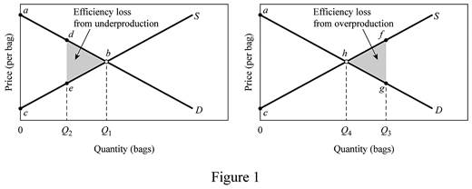
In figure -1 panel (a) and (b), the horizontal axis measures the quantity of bags and the vertical axis measures the
The inverse demand function can be derived as follows:
The inverse demand functions of
The inverse supply curve can be calculated as follows:
The inverse supply functions of
The inverse demand function and supply functions reveal that the producer willing price is $5 and the consumer willing price is $85. The equilibrium price is $45. The total surplus can be calculated as follows:
The total surplus is $800.
The consumer surplus can be calculated as follows:
The consumer surplus is $400.
Concept Introduction:
Consumer surplus: It refers to the variation in the probable charge of a product that the consumer intends to pay and the actual price that he has already paid.
Subpart (b):
The consumer surplus, total surplus and deadweight loss.
Subpart (b):
Explanation of Solution
The consumer willing price at Q2 level of output (15 units) can be calculated by substituting the Q2 level of output to the inverse demand function.
The consumer new willing price is $55.
The producer willing price at Q2 level of output (15 units) can be calculated by substituting the Q2 level of output into the inverse supply function.
The producer’s new willing price is $35.
The deadweight loss can be calculated as follows:
The deadweight loss is $50.
The total surplus can be calculated as follows:
The total surplus is $750.
Concept Introduction:
Consumer surplus: It refers to the variation in the probable charge of a product that the consumer intends to pay and the actual price that he has already paid.
Producer surplus: It refers to the variation in the probable price that the producer intends to sell and the actual price that he has already sold.
Subpart c):
The consumer surplus, total surplus and deadweight loss.
Subpart c):
Explanation of Solution
The consumer willing price at Q3 level of output (27 units) can be calculated by substituting the Q3 level of output to the inverse demand function.
The consumer new willing price is $31.
The producer willing price at Q3 level of output (127 units) can be calculated by substituting the Q3 level of output to the inverse supply function.
The producer new willing price is $59.
The deadweight loss can be calculated as follows:
The deadweight loss is $98.
The total surplus can be calculated as follows:
The total surplus is $702.
Concept Introduction:
Consumer surplus: It refers to the variation in the probable charge of a product that the consumer intends to pay and the actual price that he has already paid.
Producer surplus: It refers to the variation in the probable price that the producer intends to sell and the actual price that he has already sold.
Want to see more full solutions like this?
Chapter 4 Solutions
Microeconomics

- As indicated in the attached image, U.S. earnings for high- and low-skill workers as measured by educational attainment began diverging in the 1980s. The remaining questions in this problem set use the model for the labor market developed in class to walk through potential explanations for this trend. 1. Assume that there are just two types of workers, low- and high-skill. As a result, there are two labor markets: supply and demand for low-skill workers and supply and demand for high-skill workers. Using two carefully drawn labor-market figures, show that an increase in the demand for high skill workers can explain an increase in the relative wage of high-skill workers. 2. Using the same assumptions as in the previous question, use two carefully drawn labor-market figures to show that an increase in the supply of low-skill workers can explain an increase in the relative wage of high-skill workers.arrow_forwardPublished in 1980, the book Free to Choose discusses how economists Milton Friedman and Rose Friedman proposed a one-sided view of the benefits of a voucher system. However, there are other economists who disagree about the potential effects of a voucher system.arrow_forwardThe following diagram illustrates the demand and marginal revenue curves facing a monopoly in an industry with no economies or diseconomies of scale. In the short and long run, MC = ATC. a. Calculate the values of profit, consumer surplus, and deadweight loss, and illustrate these on the graph. b. Repeat the calculations in part a, but now assume the monopoly is able to practice perfect price discrimination.arrow_forward
- how commond economies relate to principle Of Economics ?arrow_forwardCritically analyse the five (5) characteristics of Ubuntu and provide examples of how they apply to the National Health Insurance (NHI) in South Africa.arrow_forwardCritically analyse the five (5) characteristics of Ubuntu and provide examples of how they apply to the National Health Insurance (NHI) in South Africa.arrow_forward


 Microeconomics: Principles & PolicyEconomicsISBN:9781337794992Author:William J. Baumol, Alan S. Blinder, John L. SolowPublisher:Cengage Learning